Understanding the Reflection Coefficient
 Jeffrey P. Freeman
Sep 10, 2020
16 min read
Jeffrey P. Freeman
Sep 10, 2020
16 min read
TL;DR A deep dive into the reflection coefficient ((\Gamma)): what it means physically, how to calculate SWR and load impedance from it, how feedline length affects phase, and how directional couplers measure it in practice. Today I hope to answer a rather complex question: What does the Reflection Coefficient mean exactly, how do we measure it, and what can we do with it once we do. For example if we have a reflection coefficient of \(0.
A deep dive into the reflection coefficient ((\Gamma)): what it means physically, how to calculate SWR and load impedance from it, how feedline length affects phase, and how directional couplers measure it in practice.
Today I hope to answer a rather complex question: What does the Reflection Coefficient mean exactly, how do we measure it, and what can we do with it once we do. For example if we have a reflection coefficient of \(0.5 \angle 30^{\circ}\) at at some point in a feedline what does that mean and how can we use it?
There is a lot to unpack in such a short question, there are many things the reflection coefficient can tell us on its own, and quite a few more things it can tell us when we know a few other variables.
In simplest english terms it means that the reflected wave is half the peak voltage of the forward wave, and that at any moment the reflected wave is 30 degrees ahead in its phase compared to the forward wave. So if measured on an oscilloscope comparing the waves would look something like this.
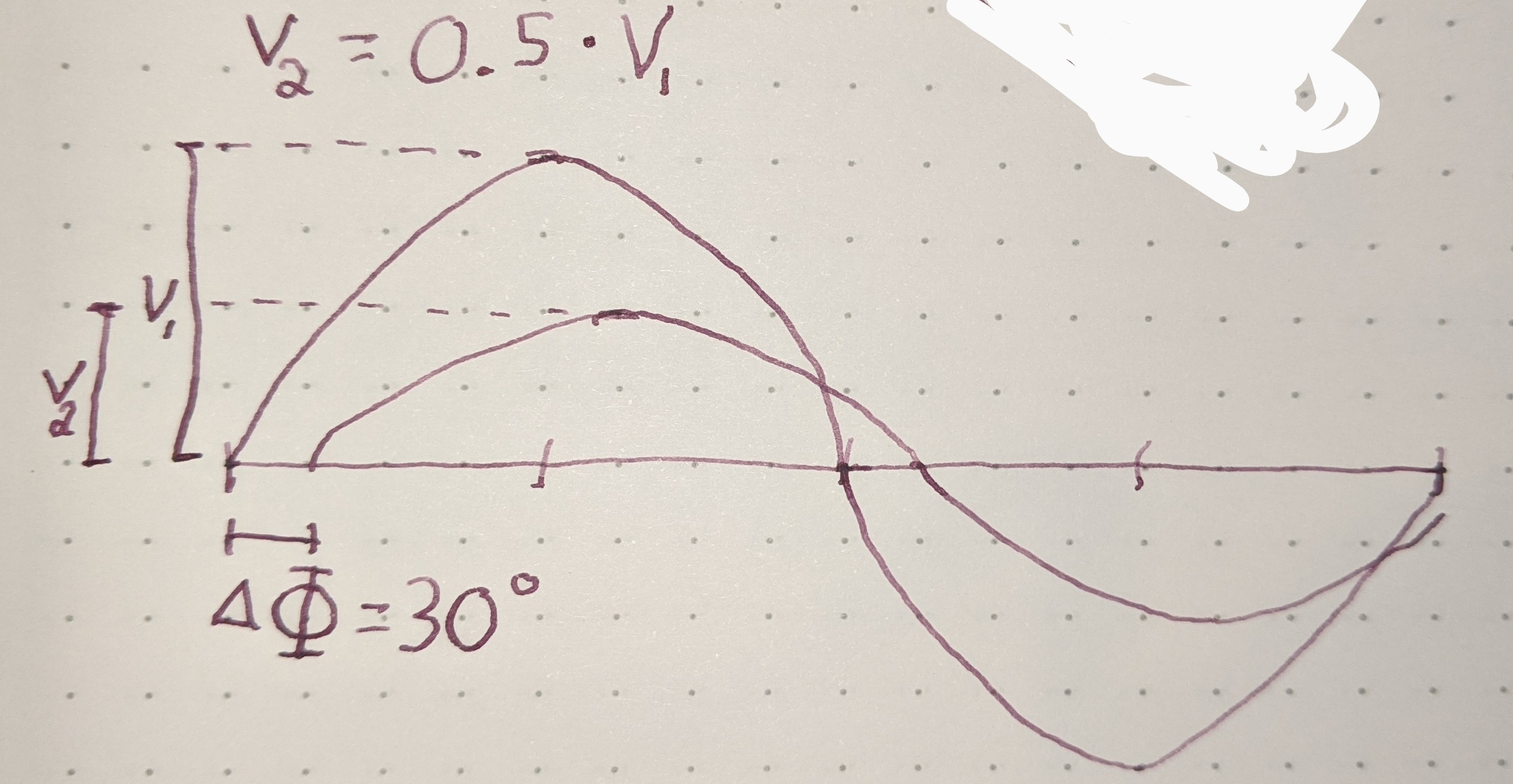
Keep in mind the waves on an oscilloscope would both be moving to the right on the display at the same speed, so they will always have the same orientation relative to each other. Meanwhile the actual waves in the feedline are moving in opposite directions so their peaks are constantly moving away from each other. Consequently this is why the phase relationship between the two waves will vary depending on the position you measure it at.
Here is what the actual waves would look like in the feedline where the x-axis here would be the position on the feedline (not to be confused with the above image that you would see on an oscilloscope).
So imagining the above image is voltage we see the green wave moving in one direction on the feedline and the blue wave moving in the opposite direction. The redline is the actual voltage at the respective point on the feedline as it changes with time. The situation here is what you would see if the far end of the feedline where the antenna should be had either an open connection or was short circuited. The red wave we see is what we call a Standing Wave. So what we are really doing when we measure the reflection coefficient is we measure the red wave in the above image at a particular point in the feedline for voltage, then do the same for current, and by comparing the two
Now let's talk a little about how knowing the reflection coefficient is useful and how you can calculate it.
Calculating \(\Gamma\)
As was already pointed out the reflection coefficient tells you the signal that is reflected relative to the forward signal. So per the example I gave at the begining you would say:
$$ \Gamma = 0.5 \angle 30^{\circ} $$
The above is in polar form but its good to remember this is little more than a complex number closely related to phasors (both voltage and current phasors). In complex form we have:
$$ \Gamma = 0.43 + 0.25 i\mkern1mu $$
Now the first thing it can tell us other than the relationship between forward and reverse voltage signals is it can also tell us the relationship between forward and reverse current signals. The relationship being the same but of opposite sign.
$$ \Gamma = -\frac{I_{refl}}{I_{fwd}} = \frac{V_{refl}}{V_{fwd}} $$
Where \(I\) and \(V\) are their respective current and voltage phasors. Remember a phasor represents the amplitude and phase of the signal relative to some reference point, usually whatever we consider ground. So from this it tells us that in our example the reflected current signal will have an amplitude of 0.5 relative to the forward current and a phase of 210 degrees, or -150 degrees whichever you'd like.
Calculating SWR from \(\Gamma\)
The other thing we can calculate directly from the reflection coefficient is the SWR, which is no longer a complex value, it's a dimensionless ratio. We lose a bit of information (the complex part) in doing this conversion but it is often a useful number used in tuning radio systems. I will explain exactly how SWR is helpful in a minute but first let's show how to calculate it.
$$ SWR = \frac{1 + \mid \Gamma \mid}{1 - \mid \Gamma \mid} $$
So again taking the initial example we would have the following SWR:
$$ SWR = \frac{1 + 0.5}{1 - 0.5} $$
$$ SWR = \frac{1.5}{0.5} $$
$$ SWR = \frac{3}{1} $$
So we would say here we have an SWR of \(3:1\) . SWR basically tells us how bad of a mismatch we have without worrying about if the mismatch is resistive or reactive. In a perfectly matched system there would be no reflected wave so your SWR is always 1:1 and thus shows us a perfect impedance match. Similarly the worst possible match we could have would be an open circuit or a short circuit, both of which would produce an infinite SWR.
Now its important to note it only tells us about what the impedance match is at the point in the circuit we measure. With a 1:1 SWR or a reflection coefficient of 0 telling us that whatever feedline and antenna is on the load end of the meter as a whole is the same impedance as the feedline and transmitter system on the source side of the meter. By itself it tells us nothing about if the antenna is well matched or well tuned, or the efficiency of the system, or even what the SWR might be at any other point in the feedline. To figure out any of that we would either need to measure at multiple points or need some more information about the components in the system.
SWR only tells us about the impedance match at the exact point where it is measured. It says nothing about antenna tuning, system efficiency, or the SWR at any other point in the feedline.
Typically SWR meters, and therefore indirectly the reflection coefficient, is useful if it is measured at the point where a transmitter connects to a long feedline which ultimately feeds some load (usually an antenna). A large mismatch at this point will cause any power a transmitter creates intended for the antenna to be reflected back into the transmitter at its outgoing port rather than making it onto the feedline. This causes that energy to be dissipated by the transmitter and ultimately will heat up the transmitter and in some cases can fry it. So it is important to have an SWR that is relatively low for the safety of the transmitter.
Relationship of Load and Source Impedance
From this point on I want to be clear on some terminology I am about to use. If I say "load impedance" I will be talking about the total impedance of the system from the point the reflection coefficient was measured all the way to the far end of the transmission line. This means we are talking about the impedance of that whole half of the system, usually a transmission line, antenna, and maybe even a tuner. It does not refer to just what is connected at the end of the transmission line itself (usually the antenna), we will get to that later. Similarly when I say "source impedance" I will also be talking about the whole system on the transmitting side of where the reflection coefficient was measured.
So with that said the other thing the reflection coefficient tells us is the relationship between the load impedance and the source impedance. The equation for that is as follows:
$$ \Gamma = \frac{Z_L - Z_S}{Z_L + Z_S} $$
Therefore if we have a transmitter that connects directly to our meter and the transmitter has a \(50\Omega\) antenna port on it then we know the source impedance is \(50\Omega\) and can then calculate the impedance of our load. So again going back to the initial example if given the situation I just explained we would calculate the load impedance as follows:
$$ \Gamma = \frac{Z_L - 50}{Z_L + 50} $$
$$ Z_L = \frac{-50 \cdot (\Gamma + 1)}{\Gamma - 1} $$
Note that if \(\Gamma\) is one the equation is undefined, but that would mean the load impedance is infinite, an open circuit.
$$ Z_L = \frac{-50 \cdot (0.43 + 0.25 i\mkern1mu + 1)}{0.43 + 0.25 i\mkern1mu - 1} $$
$$ Z_L = \frac{-50 \cdot (1.43 + 0.25 i\mkern1mu)}{-0.57 + 0.25 i\mkern1mu} $$
$$ Z_L = \frac{-71.5 - 12.5 i\mkern1mu}{-0.57 + 0.25 i\mkern1mu} $$
$$ Z_L \approx 97.1347 + 64.5328 i\mkern1mu $$
$$ Z_L \approx 116.6174610 \angle -146.401367^{\circ} $$
Relationship of Feedline Length and Phase
If we know the position on the feedline that we measured the signal relative to the far end of the load, where the antenna normally is, then we can calculate a few other meaningful things. Keep in mind in the real world the speed at which an electrical signal travels through the feedline is close to the speed of light but not quite. Each feedline is a bit different and we would look at a datasheet for our particular feedline to get what is called the Velocity Factor. This is a percentage or ratio that tells us the percentage of the speed of light a wave will propagate through the feedline. So we would calculate the actual speed of our waves as follows.
$$ c = C \cdot V_f $$
Because of this not only will the wave move slower through the feedline but it will also have a shorter wavelength than what it would when propagating through a vacuum. Let's look at the equation for wavelength real quick.
$$ \lambda = \frac{c}{f} $$
Where c is the speed of the wave through the medium as we calculated above and f is the frequency, giving us \(\lambda\) as our wavelength.
When talking about a reflection coefficient we are talking about the reflected wave relative to the forward wave. So we can consider the forward wave as our reference wave and take that as our phase reference point. We know that the reflected wave needs to travel from the point being measured to the far end of the load side and then back again, so it travels a total of twice the distance of the load side. Therefore we can calculate the phase shift with the following equation.
$$ \phi = { \frac{2 \cdot l_L}{\lambda} } \cdot 360^{\circ} $$
Where \(l_L\) is the length from the point being measured to the far end of the load, \(\lambda\) is the adjusted wavelength from earlier, and \(\phi\) is the difference in phase shift of the reflected wave relative to the forward wave. Also the curly brackets is a mathematical notation saying to take the fractional part (drop the whole number and just keep the decimal). As you can see by varying the length of the transmission line on the far side of the load we can vary the phase as we wish and thus modify our reflection coefficient to some extent.
Measuring \(\Gamma\)
One very important thing to point out here, because this is where a lot of people get things wrong. Since we are measuring a single point in the feedline we are measuring the sum of the actual forward and reverse waves at that point and we can't measure the two waves directly, all we know is how the voltage and current is changing at that one point in the line. So to say we are measuring the reflected wave at all is a bit of a lie, we are really just measuring the voltage and current values at a single point and then reconstructing the forward and reverse waves from that. While this may confuse your current understanding this is very important because this is where almost everyone goes wrong on understanding these concepts. But keep in mind just because we cant measure them directly, the two waves are still there. The following is a schematic showing a circuit called a Directional Coupler, this is how we would measure the forward and reverse waves at a point in the feedline.
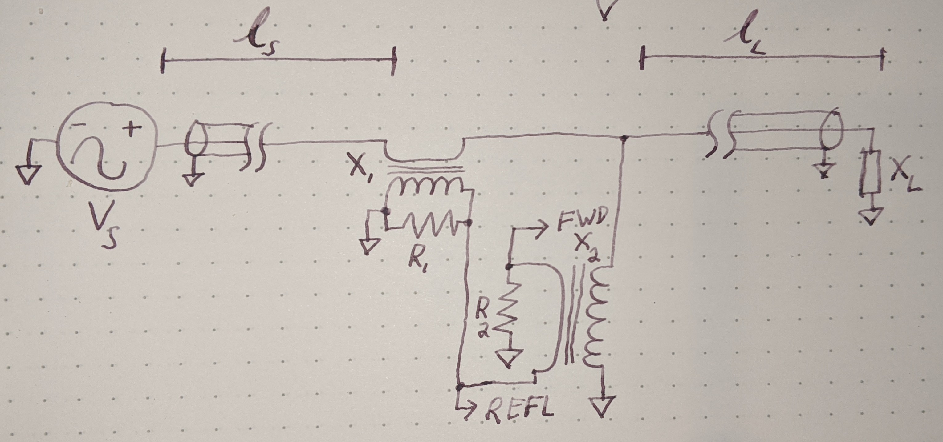
Notice from the above schematic all we are really doing is Sampling the forward current with \(X_1\) and sampling the forward voltage with \(X_2\) and then biasing the forward signal by the reflected and vice versa. This is how we reconstruct forward and reverse signals when all we know is the voltage and current at a single point.
Imagine we have a perfectly matched system where the characteristic impedance of the feedline is the same as the load and source impedance. What we would see is only a single forward moving wave, no reflected wave at all. Also, if you recall a resistor always has its current in phase with its voltage, this holds true in a matched feedline as well since all the components are real resistance with no reactance. So we would expect the forward voltage wave and the forward current wave to both be in phase without any reflected wave to interfere with them. Looking back at the above schematic we see that the \(X_2\) transformer would sample the forward voltage, which would cause the FWD output to cycle through positive and negative while the other terminal would want to swing the opposite, when fwd is high the other terminal will try to go negative, however its biased by the refl power, so we have to consider that as well. Since current is in phase and the \(X_1\) transformer is similarly going to swing inphase with the fwd port but since its connected to the opposite terminal of \(X_1\) it will essentially cancel out and the reflected port will stay at ground. However if the phase of the current and voltage were not the same then the circuit would respond very differently and we would see a signal out of the reflected port. So really the circuit is measuring the phase difference between voltage and current and using this to reconstruct the forward and reverse waves.
As an example here is what the voltage and phase relationship would look like in a feedline with an open circuit at the antenna end:
As we know impedance in its polar form has an amplitude and a phase component just like our reflection coefficient does. The phase component of an impedance value basically just tells you if you apply a voltage signal across the device how much the voltage and current signals will be out of phase with each other. A resistor always has an impedance that is equal to its resistance and has no imaginary component, and also has a phase of 0 degrees. This agrees with what I said earlier regarding a resistors voltage and current always being inphase with each other. We also know that a capacitor and the inductor always has its current 90 degrees out of phase with its voltage.
We just learned from the above schematic that the voltage-current relationship is in fact equivalent to the forward-reflected wave relationship. One can be used to determine the other and vice versa. Therefore we know that the impedance of the antenna can not just affect the amplitude of the wave it reflects back, but can also dictate its phase.
Feedline as an Impedance Transformer
We mentioned earlier how the reflection coefficient can be calculated by simply knowing the total impedance on one side of the point being measured vs that on the other side. I also pointed out how the load impedance in that calculation described the entire system on the load side including the feedline and wasn't necessarily the same as the load at the terminating end of the feedline, usually an antenna. Since we now know that the impedance of the antenna dictates not just the amplitude of the wave reflected, but also its phase, and we also know that the length of the feedline itself can shift the phase as well, it should be obvious that we can view a transmission line as an impedance transformer where the impedance of the antenna is transformed into a different impedance based on the length of the transmission line.
In essence we can tweak the load end of the transmission line by making it longer up to one wavelength and as such adjust our reflected wave's phase to whatever value we want, thus allowing us to change the reflection coefficient we see which is equivalent to changing the load side's impedance.
Going back to our original example if the reflected wave is 30 degrees out of phase lets see what would happen if we brought it inphase to 0 degrees. To do that lets calculate the length change of the feedline we would need, we will assume we are working with a wavelength of one meter.
$$ \phi = { \frac{2 \cdot l_L}{\lambda} } \cdot 360^{\circ} $$
$$ -30^{\circ} = \frac{2 \cdot l_L}{1} \cdot 360^{\circ} $$
$$ \frac{-30^{\circ}}{360^{\circ}} = 2 \cdot l_L $$
$$ \frac{-30^{\circ}}{2 \cdot 360^{\circ}} = l_L $$
$$ \frac{-1}{24} = l_L $$
So we know that if we subtract \(\frac{1}{24}\) of a meter off we will get the desired effect, or of course we could add \(\frac{23}{24}\) of a meter and get the same effect. This would change our reflection coefficient to:
$$ \Gamma = 0.5 \angle 0^{\circ} $$
or
$$ \Gamma = 0.5 + 0 i\mkern1mu $$
What is interesting is, as I said, this also changes what the load impedance looks like (the feedline plus antenna). Where before the impedance appeared mostly resistive with a small reactive component it now looks indistinguishable to our meter as a purely resistive load impedance, albeit still a mismatched one though. If we take our impedance equation from earlier and calculate it for our new reflection coefficient we can see exactly what that would be.
$$ Z_L = \frac{-50 \cdot (\Gamma + 1)}{\Gamma - 1} $$
$$ Z_L = \frac{-50 \cdot (0.5 + 1)}{0.5 - 1} $$
$$ Z_L = \frac{-50 \cdot 1.5}{-0.5} $$
$$ Z_L = \frac{-75}{-0.5} $$
$$ Z_L = 150 $$
So we effectively changed the old impedance of the load side from \(116.61 \angle -146.40^{\circ} \Omega\) to just \(150 \Omega\) , pretty neat.
Similarly we can look at this slightly differently. We can say if we know the feedline's length, and the complex impedance of the antenna, then what would be the impedance we see if we measure the antenna through the feedline. For that the equation is as follows:
$$ Z_L = Z_0 \cdot \frac{Z_{ANT} + Z_0 \cdot \tan(\frac{2\pi}{\lambda} \cdot l) i\mkern1mu}{Z_0 + Z_{ANT} \cdot \tan(\frac{2\pi}{\lambda} \cdot l) i\mkern1mu} $$
Where (Z_L) is the impedance measured through the feedline, (Z_0) is the characteristic impedance of the feedline, (l) is the length of the feedline, (\lambda) is the wavelength of the signal in the feedline, and (Z_{ANT}) is the impedance of the antenna at the far end of the feedline, or some other load.
check_circleKey takeaways
-
- The reflection coefficient \(\Gamma\) describes the amplitude and phase relationship between forward and reflected waves
- SWR is derived from \(|\Gamma|\) and indicates mismatch magnitude, but only at the measurement point
- Load impedance can be calculated from \(\Gamma\) and known source impedance
- Feedline length transforms phase, allowing a transmission line to act as an impedance transformer
- Directional couplers reconstruct forward and reverse waves from single-point voltage and current measurements
Data scientist, open-source innovator, and three-time founder who writes about graphs, radios, and the occasional impossibility. Allegedly just another data scientist. Say hello →