Nodal Analysis is a technique for circuit analysis where each node (A point where two or more components are connected) is interpreted individually. This analysis can be used to determine the voltage, or any other variable, at any point in the circuit, sometimes as a function of time. It is based on the fact that at any node all the current that enters the node will be equal to all the current leaving that same node. By doing this we are able to reduce each node to an equation, and then, the entire circuit to a set of simultaneous equations.

Identifying nodes

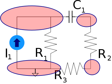
First you need to learn how to identify nodes in a circuit. A node is simply the junction where two or more components are connected by wire. The following diagram shows a circuit where the nodes are circled in red:

Analyzing a node

The next step is to represent each node in your circuit as an equation. If you are doing an analysis in the time domain then this is usually represented as voltage as a function of time \(V(t)\). This can also be done in the frequency domain using Phasors. For this example we will work in the time domain. Let's use the same circuit as the one above:

First we need to assign arbitrary directions for the current flow in and out of each component on the circuit. It doesn't need to match the direction the actual current flows because if we reverse it then the values we get for the current through that component will just come out to be negative. What is important is that if current goes in one side of a component it goes out the other side. Other than that it's completely arbitrary. So lets pick some random directions for the current flow in our diagram:

You probably also noticed the ground point. This is also arbitrary, you can pick any node in the circuit as your ground. Mathematically you represent whatever node you pick as ground to be 0 volts. Depending on which point you pick as ground it will effect the voltage values you get for the other nodes, but they will all be the same relative to each other.

Lets assume \(I_{1}\) varies with time. Therefore it will be represented as a mathematical function: \(I_{1}(t)\). Now lets look at each node individually and represent them as mathematical functions. In addition let's assign a variable to each node representing that node's voltage.

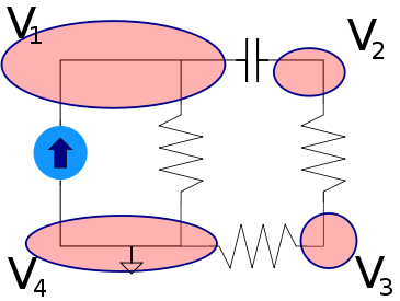
First let's look at the upper left node labeled \(V_{1}\), the one connecting \(I_{1}\), \(R_{1}\), and \(C_{1}\). It has three paths for current to flow in/out from each of the three components. We know these three currents will add up to zero because all the current coming into the node (positive values) must equal all the current exiting the node (negative values). With this knowledge we can represent the node mathematically.

The current coming in from \(I_{1}\) is easy, since this is a current source that varies with time it is simply \(I_{1}(t)\).

We then need to consider the current coming into the node from \(R_{1}\). Since we know Ohm's Law which states \(I=V/R\) we can represent the current flowing through \(R_{1}\) in these terms. Since \(V_{4}\) is our ground point it will always have a voltage of 0. Therefore the current flowing through \(R_{1}\) is simply:

$$ \frac{0-V_{1}(t)}{R_{1}} $$

Now the current through \(C_{1}\) is a bit more tricky since we need to use differential equations to model a capacitor in the time domain. The differential equation representing the current flowing through a capacitor is:

$$ I=C\frac{,dv}{,dt} $$

Therefore we represent the current through \(C_{1}\) as:

$$ C_{1}\frac{,d}{,dt}(V_{1}(t)-V_{2}(t)) $$

Remembering that the sum of these three currents will equal zero we come up with the equation:

$$ I_{1}(t)+\frac{0-V_{1}(t)}{R_{1}}-C_{1}\frac{,d}{,dt}(V_{1}(t)-V_{2}(t))=0 $$

The final step is to get this into a function representing the node's voltage as a function of time, in other words \(V_{1}(t)\). To do this we just use some calculus and differential math to solve for \(V_{1}(t)\) in the above equation. Teaching calculus is outside the scope of this document so we will leave it to the reader to solve for \(V_{1}(t)\). Once we solve for \(V_{1}\) we get the following:

$$ V_{1}(t)= \frac { ( \int\limits_0^t ( e^{-\frac{t}{C_{1}R_{1}}} ( I_{1}(t)+C_{1} ( \frac{,d}{,dt}V_{2}(t) ) ) ) ,dt )e^{\frac{t}{C_{1}R_{1}}} } {C_{1}} $$

We now know the voltage of this node (\(V_{1}\)) as a function of time. The only problem is that this function also seems to depend on the voltage functions for the other 3 nodes. That's why the next step is to obtain the voltage as a function of time for the other 3 nodes in the same way we did for this node. Once we do that we will have 4 simultaneous equations and we will have what we need to solve for any variable we want.

Lets quickly go through and perform nodal analysis on the other 3 nodes starting with node \(V_{2}\):

$$ C_{1}\frac{,d}{,dt}(V_{1}(t)-V_{2}(t))+\frac{V_{3}(t)-V_{2}(t)}{R_{2}}=0 $$

Solve for \(V_{2}(t)\) to get:

$$ V_{2}(t)=\frac{(\int\limits_0^t (e^{\frac{t}{C_{1}R_{2}}}(C_{1}R_{2}(\frac{,d}{,dt}V_{1}(t))+V_{3}(t))),dt)e^{-\frac{t}{C_{1}R_{2}}}}{C_{1}R_{2}} $$

The last two nodes will be much simpler since they don't connect to the capacitor, therefore we don't need to deal with differential equations. For \(V_{3}\) we get:

$$ -\frac{V_{3}(t)-V_{2}(t)}{R_{2}}+\frac{0-V_{3}(t)}{R_{3}}=0 $$

Solve for \(V_{3}(t)\) and you get:

$$ V_{3}(t)=\frac{R_{3}V_{2}(t)}{R_{3}+R_{2}} $$

For node \(V_{4}\) we already know its value is 0 so we can skip this node all together.

We now have 3 simultaneous equations, one for each node of the circuit (except ground). In the next section we will use them to solve for the voltage at any point as a function of time.

Bringing it all together

The rest of the process should be pretty apparent right now if you're familiar with solving for simultaneous equations. Since this isn't meant to be a math tutorial we won't go into the details on how to solve simultaneous equations.

There are basically two approaches to simultaneous equations. Either substitution, which is more tedious but doesn't require any advanced math, or linear algebra matrices. Generally if you aren't familiar with linear algebra and are doing it by hand you're gonna want to use substitution, which is the same as the process in basic algebra. However if you are familiar with linear algebra and plan to use a calculator to get your answer then matrices are much easier to work with.

The first step is to assign some values to our components (normally this is done for you of course):

$$ C_{1}=\frac{1}{100000} F $$

$$ R_{1}=100 \Omega $$

$$ R_{2}=1000 \Omega $$

$$ R_{3}=10000 \Omega $$

Similarly we need to define the function governing the current source. We will use a simple sinusoidal current source:

$$ I_{1}(t)=sin(t) $$

Since the scope of this tutorial doesn't include calculus we will show the quick way to do this in maple. To solve for multiple simultaneous equations in maple simply use the dsolve command like this:

dsolve({<equation 1>,<equation 2>,...<equation n>},[<unknown 1>, <unknown 2>,...<unknown n>])

Maple will now produce the three independent functions for the 4 nodes. When we plug the values for the components in and solve for the various nodes simultaneously we get the following equations:

$$ V_{1}(t)=100 sin(t)-\frac{100}{111} e^{-\frac{1000}{111}t}(\int\limits_0^t (cos(t)e^{\frac{1000}{111}t}) ,dt) $$

$$ V_{2}(t)=\frac{11000}{111} e^{-\frac{1000}{111}t}(\int\limits_0^t (cos(t)e^{\frac{1000}{111}t}) ,dt) $$

$$ V_{3}(t)=\frac{10000}{111} e^{-\frac{1000}{111}t}(\int\limits_0^t (cos(t)e^{\frac{1000}{111}t}) ,dt) $$

Thats all there is to analyzing a circuit in the time domain!

Jeffrey Phillips Freeman

Data scientist, open-source innovator, and three-time founder who writes about graphs, radios, and the occasional impossibility. Allegedly just another data scientist. Say hello →