Duality is an approach that has been applied across countless disciplines where one takes an existing structure and transforms it into an equivalent structure, often with the intention of making it more useful for a particular context. In electronic circuits this usually means we take an existing circuit schematic and transform it in such a way that it serves a similar purpose but suited to our specific use case. One extremely trivial example of this would be converting two resistors in series, which act as a voltage divider, into two resistors in parallel producing a current divider. Another similarly trivial example would be to take a voltage divider and double the values of its resistors such that it divides the voltage by the same ratio but uses half the current to do so. In both cases the fundamental idea of dividing a value by a given ratio is the same, we just transform the circuit in different ways that are suited to our needs.
One of the key advantages of duality is that it is feature-preserving, as such if the original circuit has particular desirable features but otherwise may not be well suited for our application we can transform the circuit into a dual in such a way as to preserve the desirable features but transform the undesirable features. For example a resistor based voltage divider has the advantageous feature of being relatively stable across various frequencies where other types of voltage dividers may have a very limited frequency range, so a resistor based voltage divider may be best suited for an extremely broadband application (large range of frequencies). However our application may require low-power consumption and the voltage divider may not need to drive a load and only need to be provided as an input to an IC with high impedance. As such if our reference circuit is for a voltage divider that uses relatively small values for resistors, and thus draws too much power, we can transform the voltage divider into its dual that preserves the frequency-stability of the original but reduces the current draw. This of course is a very trivial example, the concept of duality can, and often is, applied to much larger complex circuits as well. For this reason understanding circuit duality, and duality in general, specifically how to recognize it, apply it, and common circuit applications is a vital tool in anyone's mental toolbox.
What is a Dual?
Duality is the transformation of a mathematical model or structure into an equivalent mathematical model or structure such that each element of the original has a one-to-one relationship with an element in the result. The transformation between its elements usually represents an involution, which means if the same transformation is applied twice you wind up with the original; at the very least the transformation must be reversible (invertible) back to its original form. This implies that the transformation must be unique for any given input. Both the overall structure once converted is said to be the dual of the original, but so too are the individual elements of the structure considered the dual of their counterpart in the dual structure.
Taking the reciprocal is an example of an involution, and thus a trivial example of duality.
\(\definecolor{current}{RGB}{0, 255, 221}\) \(\definecolor{voltage}{RGB}{181, 181, 98}\) \(\definecolor{impedance}{RGB}{18,110,213}\) \(\definecolor{resistance}{RGB}{114,0,172}\) \(\definecolor{reactance}{RGB}{45,177,93}\) \(\definecolor{imaginary}{RGB}{251,0,29}\) \(\definecolor{capacitance}{RGB}{255, 127, 0}\) \(\definecolor{inductance}{RGB}{255,0,255}\) \(\definecolor{permeability}{RGB}{0,255,0}\) \(\definecolor{permittivity}{RGB}{255,0,0}\) \(\definecolor{normal}{RGB}{0,0,0}\)
$$ f(x) = \frac{1}{x} $$
Since \(f(x)\) is an involution the following must be true for any involution function.
$$f(f(x)) = x$$
Of course for the reciprocal this holds true.
$$x = 5$$
$$f(5) = \frac{1}{5}$$
$$f(\frac{1}{5}) = 5$$
Therefore we can say \(5\) is the dual of \(\frac{1}{5}\) under the reciprocal transformation.
An involution can sometimes be an identity function, and thus create fixed points where the involution of one element is unchanged. This of course still holds true to the rules of a duality transformation whereby if the involution is applied twice you still wind up at the original, it is invertible. The identity transformation would be:
$$ f(x) = x $$
Therefore it is trivial to see this holds true as an involution since the following is true.
$$ f(f(x)) = x $$
In this case any value is the dual of itself under the identity transformation. Which isn't really saying much, but it is important to understand a fixed point is still a dual caused by an involution.
As stated earlier duals are usually transformed between each other through an involution function, but this does not need to be the case. Any invertible (reversible) function can be a valid way to express duality. The technical term for the property of a function to be reversible is to say it is bijective But this is just a fancy way of saying you can reverse the function to get to where you started. For example adding one to a value is a bijective function since you can also subtract one and always get to where you started and there is no ambiguity in doing so. However multiplying by 0 is not bijective (invertible) because once you multiply by 0 you have no way of getting back to where you started, all numbers would transform into 0. In other words in order for a function to be invertible the output of the function must be a unique value for any given input of the function, otherwise ambiguity is introduced and there would be no way to reverse the process.
$$ f(x) = x + 1 \label{addone}$$
As stated equation \(\eqref{addone}\) is invertible as you can always subtract \(1\) and get back to where you started.
$$ f^{-1}(x) = x - 1 $$
$$ f^{-1}(f(x)) = x \label{inv} $$
In this case \(f^{-1}(x)\) is called the inverse function to \(f(x)\) and the notation used in equation \(\eqref{inv}\) is the typical notation used to represent an inverse function. It should be trivially obvious but keep in mind an inverse function must work in both directions, in other words.
$$ f(f^{-1}(x)) = f^{-1}(f(x)) = x $$
It should be noted that an involution function is closely related to a function and its inverse. All an involution function really is is a function where its inverse is itself.
Also bear in mind not all values will have a dual, consider the reciprocal function, which is an involution (its own inverse) and thus a valid transformation.
$$ f(x) = f^{-1}(x) = \frac{1}{x} $$
In the case of the reciprocal function a value of 0 for x is undefined since you can not divide by 0, any other real value other than 0, however, is valid. Therefore we can say that under the reciprocal transformation all real number values have a dual except for 0, which does not have a dual.
Examples of Duals
There are many common examples of duals in almost every subject from philosophy, to mechanical engineering, it is a pervasive idea that can often be useful in many fields. Here are a few example values and their duals under different inversion transformations.
- True is the dual of False under the negation transformation
- 10 is the dual of 0.1 under the reciprocal transformation
- 5 is the dual of -5 under the negation transformation.
- A current divider circuit is the dual of a voltage divider circuit under series-parallel transformation
- A capacitor based high-pass filter is the dual of an inductor based high-pass filter under reciprocal impedance transformation
- A bandpass filter is the dual of a band-stop filter under series-parallel transformation
- Position is the dual of velocity under the derivative/integral transformation
- Up is the dual of Down under vertical flip transformation
- In philosophy the mind is the dual of the physical world under dual-aspect theory
Similarly here are some examples of transformations and their inverse that are therefore capable of producing duals
- Reciprocal transformation is its own inverse, an involution.
- Negation transformation is its own inverse, an involution.
- derivative transformation is the inverse of an integral transformation
- A geometric flip transformation is its own inverse, an involution
- doubling a value is the inverse of halving a value
The Dual of a function
Just as we have shown above that individual variables and values have a dual under an invertible function, likewise functions can also have duals in the same manner. Imagine we have an invertible function \(T(x)\) which will convert something to its dual, and we have some function \(f(x)\) we wish to find the dual of, then simply by passing the function into T we can produce its dual. Specifically \(T(f(x)) = f^T(x)\) where the functions \(f(x)\) and \(f^T(x)\) are duals of each other. It is important to note here only \(T(x)\) needs to be invertible; neither \(f(x)\) nor \(f^T(x)\) needs to have this property. For example; say the transformation under which we create the duals is the reciprocal function, which is invertible, but \(f(x)\) is the square function, which is not invertible. We know it isn't invertible because 10 squared is 100 and -10 squared is also 100. So there is no way to reverse the value of 100 and get the original value since some information was lost, we no longer know if the original value was positive or negative.
$$T(x) = \frac{1}{X}$$
$$f(x) = x^2$$
$$f^T(x) = T(f(x)) = \frac{1}{x^2}$$
We can now see the function \(f(x) = x^2\) is the dual of \(f^T(x) = \frac{1}{x^2}\) under the reciprocal transformation.
Manipulating A System of Equations
Things get slightly more complicated when we start talking about systems rather than single variables or functions. A system is a collection of variables where some or all of the variables are dependent on the others; in other words, two or more mathematical functions dictate the value of one or more variables in relationship to other variables. In fact if you're reading this blog you are already familiar with one very important type of system we all care about, an electrical circuit. In an electrical circuit, the variables are things like the voltage{: style="color: rgb(181, 181, 98)"} at various points in the circuit and the system of functions are the electrical components that connect these points.
Mapping a System of Equations
From this point on we need a good way to visualize systems of equations so I can do a better job talking about them. So I want to describe a graphical language for diagramming systems of equations. Let's start with a simple generic component that provides an impedance{: style="color: rgb(18, 110, 213)"}, doesn't matter just yet if it's a resistor or something else. The following is a simple schematic of a lone component where some of the variables we care about are labeled.
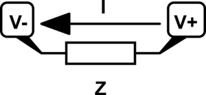
Keep in mind when we talk about Ohm's Law, we usually talk about the voltage{: style="color: rgb(181, 181, 98)"} across a component but here I have separated out the voltage{: style="color: rgb(181, 181, 98)"} on each terminal instead; it will make things a little more straight forward. Just keep in mind the voltage{: style="color: rgb(181, 181, 98)"} across the component is simply \(\color{voltage}V_+\color{normal} - \color{voltage}V_-\color{normal}\) in this case. Let's represent that component in terms of Ohm's Law which will give us the relationship between its voltage{: style="color: rgb(181, 181, 98)"}, impedance{: style="color: rgb(18, 110, 213)"}, and current{: style="color: rgb(0, 255, 221)"}. I will intentionally arrange the equation in such a way that doesn't give any one variable preferential treatment by solving for 0, this is to emphasize the fact that it is a relationship between all of the variables.
$$ \color{current}I\color{normal} \cdot \color{impedance}Z\color{normal} + \color{voltage}V_-\color{normal} - \color{voltage}V_+\color{normal} = 0 $$
The way I want to diagram an equation such as this would be as follows.

In this diagram we have variables in circles, these can have any arbitrary name and dont need to be the same name as the variables in the equations (you will see why that is necessary soon). The rectangles contain the equation, and the lines that connect it associate the shared variables, in circles, with the local variables defined in the equation. So here we have the variable \(W\) associated with \(\color{current}I\color{normal}\) for example. Lets apply this to a slightly more complex example, a simple voltage{: style="color: rgb(181, 181, 98)"} divider circuit.
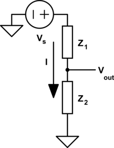

As you can see here we now have two equations, one for each component in our circuit which is capable of relating every variable/point in our circuit to every other. Some variables like current{: style="color: rgb(0, 255, 221)"} are shared between both components and relate to the same local variable in each equation. However others, like \(\color{voltage}V_{out}\color{normal}\), are also shared between both components, and both equations, but represents a different variable in each equation. This is the reason we needed to pick the specific format for our diagrams where the shared variables depicted in circles often have different names from the local variables in the equations. One important rule these diagrams will always follow is that the number of lines that connect to any particular equation will be exactly equal to the number of variables in the equation. Also note that at this stage we don't make any distinction between if a variable is a constant, or an unknown, every variable is treated the same. We will call this form of the diagram the variable relationship diagram as it shows the relationship between variables.
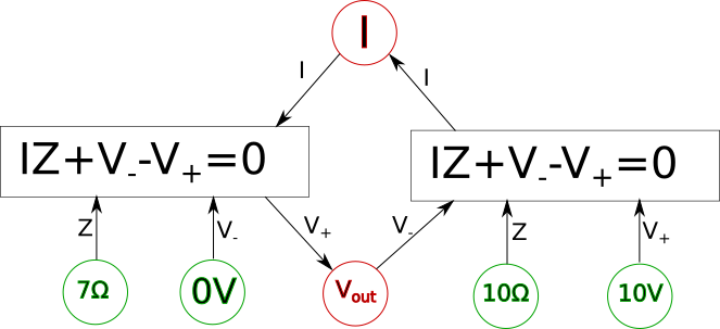
The diagram as it stands now, however, is only the first step if we want to actually solve for the variables and, for example, determine the actual voltage{: style="color: rgb(181, 181, 98)"} at \(\color{voltage}V_{out}\color{normal}\); for that we need to actually figure out what variables have known quantities, and the relationship between them. The first step to do that is to pick whichever variables have known values and plug in the actual values for those variables into the circles. We also need to change the lines in the diagram into one-directional arrows. Any known variables will always have all of the connections facing outward. Presuming we know the source voltage{: style="color: rgb(181, 181, 98)"} and the impedance{: style="color: rgb(18, 110, 213)"} of our two components lets fill in some arbitrary values now and show how that might look.

Here the known variables are highlighted in green, the unknown variables are highlighted in red, and the appropriate arrows were added. Notice we have two shared variables left, since we have two simultaneous equations we already know these can be treated as unknowns and solved for. Since in the convention we are using an arrow pointing into an equation is a variable that will be plugged into it, then an arrow pointing out of an equation will be a value the equation will solve for. As we know we can solve for any single variable in an equation and as long as all the other variables are known then we can turn our equation into a function and solve it. For example we could rearrange our equation into the following function.
$$ \color{voltage}I \cdot Z\color{normal} + \color{voltage}V_-\color{normal} - \color{voltage}V_+\color{normal} = 0 $$
$$ \color{voltage}V_+\color{normal} = \color{voltage}I \cdot Z\color{normal} + \color{voltage}V_-\color{normal} $$
All we did was isolate the \(\color{voltage}V_+\color{normal}\) on one side of the equation and now it is a function. We can represent this in our diagram by making a rule for ourselves such that when we are trying to solve for a system of equations every equation in a box in our diagram should have one and only one outgoing arrow and all other arrows should be incoming. The outgoing arrow simply represents which of the variables we are choosing to solve for in the local equation. The other rule is that any unknown we can solve for must have at least one (and usually only one) incoming arrow and the rest of the arrows are outgoing. Finally, all lines must be converted to arrows. If we can follow these stated rules and ensure each unknown we care about has an incoming arrow then the system of equations should be solvable. For example here is what the final solvable diagram would look like in this case.
Keep in mind in the above diagram there is more than one way we could have made the system solvable and still followed the outlined rules. For example the arrows connected to \(\color{voltage}V_{out}\color{normal}\) could have been reversed along with the arrows connection to \(\color{current}I\color{normal}\) also being reversed in which case we would also have had a solvable system of equations. We will call this final form of the diagram the variable dependency diagram.
Lets recap real quick the rules for a variable relationship diagram:
- Each equation, denoted by a rectangular box, should have exactly one line for each variable in the equation.
- Each global variable, denoted by a circle, should have one line connecting it to each equation it is used in.
- Lines can only connect variables (circles) with equations (rectangles)
- The variable name next to a line should match one of the variable names in the equation it connects to.
- The global variable name depicted inside a circle does not need to match the variable name on a line that connects it, but it is allowed to.
- At this stage none of the lines should have arrows associated with it.
Similarly lets recap the rules for a variable dependency diagram:
- Rules 1 through 5 above also apply here.
- All lines in the diagram should be depicted as one-directional arrows.
- For each equation in diagram one and only one line should be an outgoing arrow, all other arrows should be inbound.
- All known global variables, depicted with a circle, should have all of its lines as outgoing arrows only.
- All unknown global variables, depicted with a circle, should have at least one, and usually only one, incoming arrow, all others should be outgoing. If this rule can not be satisfied then the system is not solvable.
- There may be more than one configuration that satisfies the above rules, if so pick any arbitrary layout capable of satisfying the rules.
Let's finish up by actually solving for the unknowns in the above variable dependency diagram.
First let's take the left-hand equation.
$$ \color{voltage}I \cdot Z\color{normal} + \color{voltage}V_-\color{normal} - \color{voltage}V_+\color{normal} = 0 $$
$$ \color{voltage}I \cdot 7\Omega\color{normal} + \color{voltage}0V\color{normal} - \color{voltage}V_{out}\color{normal} = 0 $$
$$ \color{voltage}V_{out}\color{normal} = \color{voltage}I \cdot 7\Omega\color{normal} + \color{voltage}0V\color{normal} $$
$$ \color{voltage}V_{out}\color{normal} = \color{voltage}I\cdot 7\Omega\color{normal} $$
This now represents the value of \(\color{voltage}V_{out}\color{normal}\) which can then be used when we solve the right-hand equation.
$$ \color{voltage}I \cdot Z\color{normal} + \color{voltage}V_-\color{normal} - \color{voltage}V_+\color{normal} = 0 $$
$$ \color{voltage}I \cdot 10\Omega\color{normal} + \color{voltage}I \cdot 7\Omega\color{normal} - \color{voltage}10V\color{normal} = 0 $$
$$ \color{voltage}I \cdot 10\Omega\color{normal} + \color{voltage}I \cdot 7\Omega\color{normal} = \color{voltage}10V\color{normal} $$
$$ \color{voltage}I \cdot (10\Omega + 7\Omega)\color{normal} = \color{voltage}10V\color{normal} $$
$$ \color{voltage}I \cdot 17\Omega\color{normal} = \color{voltage}10V\color{normal} $$
$$ \color{current}I\color{normal} = \color{current}\frac{10}{17}A \color{normal}$$
Now that we have solved for \(\color{current}I\color{normal}\) we can finish solving the left-hand equation where we left off.
$$ \color{voltage}V_{out}\color{normal} = \color{voltage}I \cdot 7\Omega\color{normal} $$
$$ \color{voltage}V_{out}\color{normal} = \color{voltage}\frac{10}{17}A \cdot 7\Omega\color{normal} $$
$$ \color{voltage}V_{out}\color{normal} = \color{voltage}\frac{70}{17}V\color{normal} $$
$$ \color{voltage}V_{out}\color{normal} = \color{voltage}4 \frac{2}{17}V\color{normal} $$
Easy right?
Manipulating a Variable Relationship Diagram
One thing we also need to know how to do is manipulate the variable relationship diagram, which is exactly the same as manipulating a system of equations. Obviously if we have two equations that share a common variable we can combine them into a single equation which eliminates the common variable by simple substitution. A simple example of that is as follows.
$$ f = 2x+t $$
$$ t = 7+y $$
These can be combined into:
$$ f = 2x + 7 + y \label{combined}$$
Notice the variable \(t\) disappears when we do this. Of course the same is true in reverse, we can pull out some terms in an equation, replace it with a variable, and get two new equations as a result and one additional variable. For example in the equation \(\eqref{combined}\) we can pull out \(7 + y\) as a term, replace it with \(t\) and wind up with the two equations we started with.
We can likewise do the same with our variable relationship diagram, afterall it is just a way of visualizing systems of equations. Let's say we took our earlier example of a voltage{: style="color: rgb(181, 181, 98)"} divider and its corresponding variable relationship diagram. The following is what it would look like if we split up the equation \(\color{voltage}I \cdot Z\color{normal} + \color{voltage}V_-\color{normal} - \color{voltage}V_+\color{normal} = 0\) by pulling out the \(\color{voltage}I \cdot Z\color{normal}\) term and replacing it with a new variable we will call \(\color{voltage}V\color{normal}\).

Here we can see two new shared variables are created, one called \(\color{voltage}V_1\color{normal}\) and the other \(\color{voltage}V_2\color{normal}\), both represent the voltage{: style="color: rgb(181, 181, 98)"} across their respective components. Other than the addition of two new variables, and changing 2 equations into four, this diagram still represents the same voltage{: style="color: rgb(181, 181, 98)"} divider as before. It can often be useful to break up equations in this way when we are considering how to construct duals for a system of equations, but we will get to that later. Usually what we find though is breaking up equations into smaller ones is only useful down to three variables, anymore than that and we just get long chains that add a lot of verbosity to the diagram but don't really add much value beyond that. So typically when transforming to a dual we start by representing a system with three-variable equations and then we can make it more compact as we work with it.
One interesting aspect of working with things visually is it gives us clues as to which equations can be combined simply due to how the diagram is laid out. For example if you start at any equation and draw a path following the connecting lines and variables to any other equation, even if you go through multiple equations in the diagram to get there, then the path you created can be combined into a single equation. For example if we create a vertical path between the pair of equations \(\color{voltage}I \cdot Z\color{normal} - \color{voltage}V\color{normal} = 0\) up to \(\color{voltage}V\color{normal} + \color{voltage}V_-\color{normal} - \color{voltage}V_+\color{normal} = 0\) then those two paths can combine the equations and we would wind back at where we started before we split the equations up. Likewise we can also create a path starting at any of the four equations creating a loop through the other three such that the path goes through all four equations and in doing so can compact all four equations into one big equation. In fact being able to combine all the equations into one big equation is always possible as long as the system of equations we are representing is solvable.
The Dual of a Circuit
Now lets reiterate what we said earlier when we defined what a dual is: The transformation of a mathematical model or structure into an equivalent model or structure such that each element of the original has a one-to-one relationship with an element in the result, where the transformation between its elements is invertible.
At this point it should be obvious that when we talk about a mathematical model it is analogous to a system of equations, and for our focus here the equations describe an electrical circuit. Let's take a minute and consider what our definition of a dual means when we talk about a circuit. We are saying that a dual of a circuit must be functionally equivalent, in other words it is at least partially feature-preserving, and each of its components must have a one-to-one relationship between the circuits. This doesn't necessarily mean the dual will have the same components or that the voltage{: style="color: rgb(181, 181, 98)"}, current{: style="color: rgb(0, 255, 221)"}, resistance{: style="color: rgb(114,0,172)"}, or any other value, will be the same in one circuit or its dual, however they do need a one-to-one relationship where some value at some point in one circuit can serve the same function at some point in the dual of that circuit. For example if we create a dual circuit and find the output of the circuit is inverted from the original then that is acceptable since it can be seen as representing the same information in a different but equivalent way. In other words for every one-to-one relationship in a circuit and its dual, the values or components in each must also be duals of each other. In fact that's all the dual of a system really is, some system where you replace part or all of the system with its dual in such a way that the utility of the overall system is preserved.
The Circuit Dual Under Reciprocal Impedance
There are many different types of circuit duals and even more types of duals in the general sense. The most commonly taught circuit dual is the reciprocal impedance{: style="color: rgb(18, 110, 213)"} circuit dual. In this form of dual circuit each component is replaced with an equivalent component that has reciprocal impedance{: style="color: rgb(18, 110, 213)"} characteristics. Simultaneously power sources such as batteries have their polarity reversed. This will result in a dual circuit where the amplitude of the signals at any point in the circuit is unchanged but are in different locations in the new circuit. If you flip the components around the power source however instead of flipping the power source, which is functionally the same thing, the position of the voltage{: style="color: rgb(181, 181, 98)"} points will remain unchanged; which tends to be a more convenient way to visualize it. The phase of the signals, as well as the current{: style="color: rgb(0, 255, 221)"}, at any point undergoes a transformation however and is not preserved. Generally forward phase shifts become negative phase shifts of the same degree. In this type of circuit inductors become the dual of capacitors as they always have reciprocal impedance{: style="color: rgb(18, 110, 213)"} of each other for the same value component.
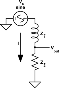
The type of circuit dual here, the dual under reciprocal impedance{: style="color: rgb(18, 110, 213)"}, is typically the type of Dual that is intended when an electrical engineer talks about a circuit dual. Let's start with a really simple example to show what we mean, consider the following RC circuit that acts as a low-pass filter.
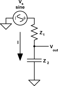
It should be apparent right away that this is very similar to our voltage{: style="color: rgb(181, 181, 98)"} divider from before except that now instead of specifying some generic unnamed components we are defining \(\color{impedance}Z_1\color{normal}\) to be the value from a resistor and \(\color{impedance}Z_2\color{normal}\) to be the value from a capacitor. This will function as a low pass filter allowing low frequency signals from \(\color{voltage}V_s\color{normal}\) to pass relatively unattenuated out of \(\color{voltage}V_{out}\color{normal}\) while attenuating higher frequency signals. A DC signal will pass through completely unaffected and as the frequency increases less of the signal will make it out.
For those of you who are familiar with this circuit you probably already know there is another way you can construct a low-pass filter that is very similar but uses an inductor in place of a capacitor. That circuit would look like this.
Assuming the correct values are picked for the components in each of these circuits then these two circuits will behave similarly and either circuit would be an effective low-pass filter.
In this case these two circuits are what we would call duals of each other whereby the inductor is the dual of the capacitor, the position of the two components are reversed, but everything in one circuit has a one to one relationship with the other one. This is one of the simplest examples of a circuit dual. Similarly the system of equations that describe these two circuits will also be duals of each other, let's take a look at that.
Since the above two circuits are essentially voltage{: style="color: rgb(181, 181, 98)"} dividers, where the impedance{: style="color: rgb(18, 110, 213)"} of the capacitor and inductor change according to frequency, we can describe both systems using a similar set of equations as we did above, just with a bit of extra detail. Let's start by looking at the system of equations that would describe the capacitor based low-pass filter. We already know the impedance{: style="color: rgb(18, 110, 213)"} of a resistor is simply its resistance{: style="color: rgb(114,0,172)"}, the impedance{: style="color: rgb(18, 110, 213)"} of a capacitor is as follows.
$$\color{impedance}Z_2\color{normal} = \color{impedance}\frac{1}{2\pi f C j}\color{normal} = \color{reactance}-\frac{1}{2\pi f C}\color{imaginary}j\color{normal} $$
Where
\(f\) is the frequency applied in Hz,
\(\color{capacitance}C\color{normal}\) is capacitance{: style="color: rgb(255, 127, 0)"} in Farad, and
\(\color{imaginary}j\color{normal}\) is the imaginary{: style="color: rgb(251,0,29)"} number.
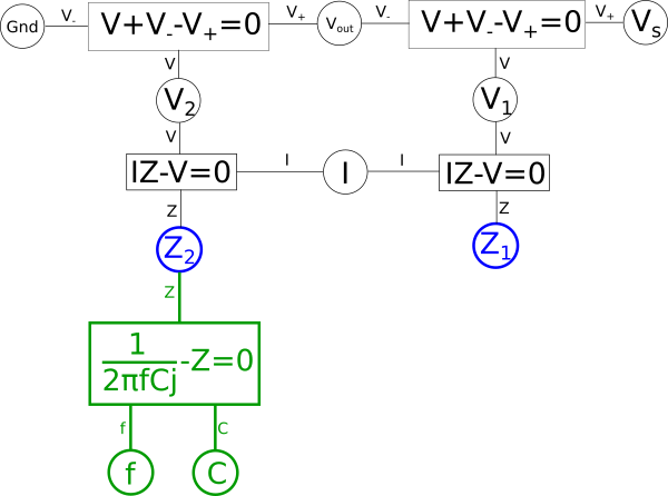
If complex numbers confuse you don't worry, for the most part for what we will be discussing you can simply ignore the imaginary{: style="color: rgb(251,0,29)"} number. If we apply this to our earlier variable relationship diagram then it would look something like this.

If we want to create a dual for the circuit represented by the above variable relationship diagram we can start by rearranging the diagram following certain rules. Keep in mind, however, that in the context here the system of equations we are working with is intended to represent a circuit. If we were dealing with a pure system of equations, that were not intended to represent something physical like a circuit, then we would have a great deal of freedom in the sorts of duals we could create by rearranging the system of equations. But since we are specifically interested in talking about circuits, we need to be mindful that any rearrangement we do can actually be represented as a circuit in the real world, it is more than just a lump of equations on a piece of paper. One simple mental check you can do when working with physical systems, like a circuit, is when creating a dual make sure when you move something around that the units associated with the various variables still make sense. If \(\color{impedance}Z_1\color{normal}\) is an impedance{: style="color: rgb(18, 110, 213)"} you can't just go plugging it into an equation for a variable where voltage{: style="color: rgb(181, 181, 98)"} is expected, for example, that just wouldn't make much sense.
The other important factor to consider here is that because we are talking about a dual, and because a dual needs to maintain a one-to-one relationship between elements of its dual, we need to ensure that all of the relevant elements in our circuit are represented in our variable relationship diagram. This means that at a minimum there should be one shared variable representing the voltage{: style="color: rgb(181, 181, 98)"} at each node in our circuit, here those would be \(\color{voltage}Gnd\color{normal}\), \(\color{voltage}V_{out}\color{normal}\), and \(\color{voltage}V_s\color{normal}\). We also need to represent the current{: style="color: rgb(0, 255, 221)"} for each mesh in the circuit; since our circuit here is just a single loop we only have one variable representing current{: style="color: rgb(0, 255, 221)"}, \(\color{current}I\color{normal}\). Naturally since the components themselves represent impedances{: style="color: rgb(18, 110, 213)"}, and ultimately the components will be what get manipulated in order to create our dual, it is useful to also insure the impedance{: style="color: rgb(18, 110, 213)"} for each component is represented in our diagram as well; here we have \(\color{impedance}Z_1\color{normal}\) and \(\color{impedance}Z_2\color{normal}\) doing just that.
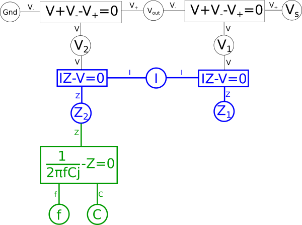
One way we can create a dual from our variable relationship diagram is to pick two shared variables of the same type, such as impedances{: style="color: rgb(18, 110, 213)"}, with the intention of flipping their positions. In this case we want to flip the impedance{: style="color: rgb(18, 110, 213)"} of our two components so we will pick \(\color{impedance}Z_2\color{normal}\) and \(\color{impedance}Z_1\color{normal}\) to be flipped to create our dual. Let's color that in our diagram blue. At the same time take any equations connected to the selected nodes that do not lie between some path between the nodes and color them green. For example the equation for the impedance{: style="color: rgb(18, 110, 213)"} of a capacitor fits that description so we will color it green, however, the equation \(\color{voltage}I \cdot Z\color{normal} - \color{voltage}V\color{normal} = 0\) does lie on a path between the two blue nodes, so we will not color it green. Next, repeat the process such that everything you just colored green has everything attached to it that is not already colored changed to green as well; repeat until there is nothing left to color. When we are done the parts colored green should not lie on a path between the two blue points. After this the diagram would be as follows.
The areas in green in our graph are the parts we intend to flip across the blue shared variables. The next step is to start at each of the two shared variables colored in blue, in this case \(\color{impedance}Z_1\color{normal}\) and \(\color{impedance}Z_2\color{normal}\), and find the shortest path between them and color it blue. We want to ensure that every non-green line connected to these variables is blue when we are done; if needed we may need to pick more than one path to accomplish that, but using the least number of paths to do so is ideal. In this case we can select a single path and satisfy that condition.
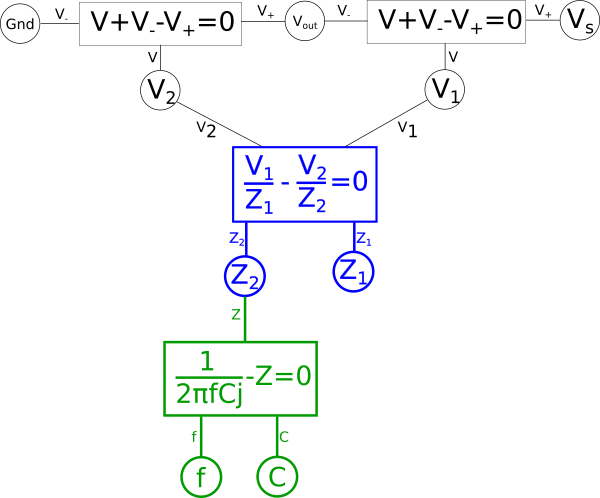
Next combine the equations in blue into a single equation.
$$ \color{voltage}I \cdot Z\color{normal} - \color{voltage}V\color{normal} = 0$$
$$ \color{voltage}I \cdot Z\color{normal} = \color{voltage}V\color{normal} $$
$$\color{current}I\color{normal} = \color{current}\frac{V}{Z}\color{normal}$$
$$\color{current}\frac{V_1}{Z_1}\color{normal} = \color{current}\frac{V_2}{Z_2}\color{normal}$$
$$ \color{current}\frac{V_1}{Z_1}\color{normal} - \color{current}\frac{V_2}{Z_2}\color{normal} = 0 $$
Giving us the following diagram.
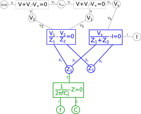
This of course creates a problem, we eliminated the global variable for current{: style="color: rgb(0, 255, 221)"}, \(\color{current}I\color{normal}\), and as stated earlier when creating duals we care about the value of \(\color{current}I\color{normal}\) so we need to add it back somewhere else in the system of equations. There are multiple places we can add \(\color{current}I\color{normal}\) back into our equation, for example the voltage{: style="color: rgb(181, 181, 98)"} across either of our two components in the circuit, divided by the impedance{: style="color: rgb(18, 110, 213)"} of that component, would give us \(\color{current}I\color{normal}\); as such we could create the equation for that and connect the \(\color{voltage}V_2\color{normal}\) shared variable and the \(\color{impedance}Z_2\color{normal}\) shared variable to it and add \(\color{current}I\color{normal}\) hanging off in our diagram on the left side. We can also do the same on the right side for the other component and get the same value of \(\color{current}I\color{normal}\). However if we did it this way we would find we would need to rearrange the diagram because if you recall the rules earlier when we defined our paths, colored in blue, this would mean we would have to create an additional path through the new equation. The path in either of those cases would mean we would have to combine and manipulate the additional path in the same way we are currently doing with the one path we have. Therefore the easier way to add \(\color{current}I\color{normal}\) back for our purposes is as a relationship between our two impedances{: style="color: rgb(18, 110, 213)"} and \(\color{voltage}V_s\color{normal}\) with the following equation.
$$\color{current}I\color{normal} = \color{current}\frac{V_s}{Z_1 + Z_2}\color{normal}$$
$$\color{current}\frac{V_s}{Z_1 + Z_2}\color{normal} - \color{current}I\color{normal} = 0$$
This equation is just Ohm's law applied to the whole circuit with the voltage{: style="color: rgb(181, 181, 98)"} across the circuit being \(\color{voltage}V_s\color{normal}\) and the total impedance{: style="color: rgb(18, 110, 213)"} of the circuit being the sum of our two individual impedances{: style="color: rgb(18, 110, 213)"}. Defining it in this way isn't necessary but it will save us the headache of doing additional work manipulating our diagram to get it into the proper form to calculate our dual.
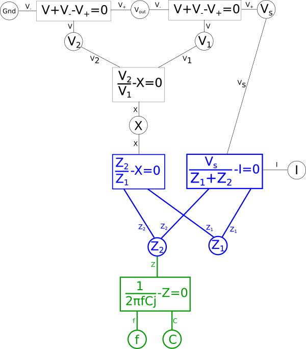
Next if the combined equation has more than three variables associated with it, split out the variables that are not part of the path. Let's start with the equation on the right hand side, in that equation we want to split out \(\color{voltage}V_1\color{normal}\) and \(\color{voltage}V_2\color{normal}\).
$$ \color{current}\frac{V_1}{Z_1}\color{normal} - \color{current}\frac{V_2}{Z_2}\color{normal} = 0 $$
$$ \color{current}\frac{V_1}{Z_1}\color{normal} = \color{current}\frac{V_2}{Z_2}\color{normal} $$
$$ \color{voltage}\frac{V_1 \cdot Z_2}{Z_1}\color{normal} = \color{voltage}V_2\color{normal} $$
$$ \frac{\color{impedance}Z_2\color{normal}}{\color{impedance}Z_1\color{normal}} = \frac{\color{voltage}V_2\color{normal}}{\color{voltage}V_1\color{normal}} $$
$$ \frac{\color{impedance}Z_2\color{normal}}{\color{impedance}Z_1\color{normal}} - \frac{\color{voltage}V_2\color{normal}}{\color{voltage}V_1\color{normal}} = 0 $$
$$ \frac{\color{impedance}Z_2\color{normal}}{\color{impedance}Z_1\color{normal}} - X = 0 $$
That is one equation, and the second:
$$ X = \frac{\color{voltage}V_2\color{normal}}{\color{voltage}V_1\color{normal}} $$
$$ \frac{\color{voltage}V_2\color{normal}}{\color{voltage}V_1\color{normal}} - X = 0$$
Again lets apply this to our diagram
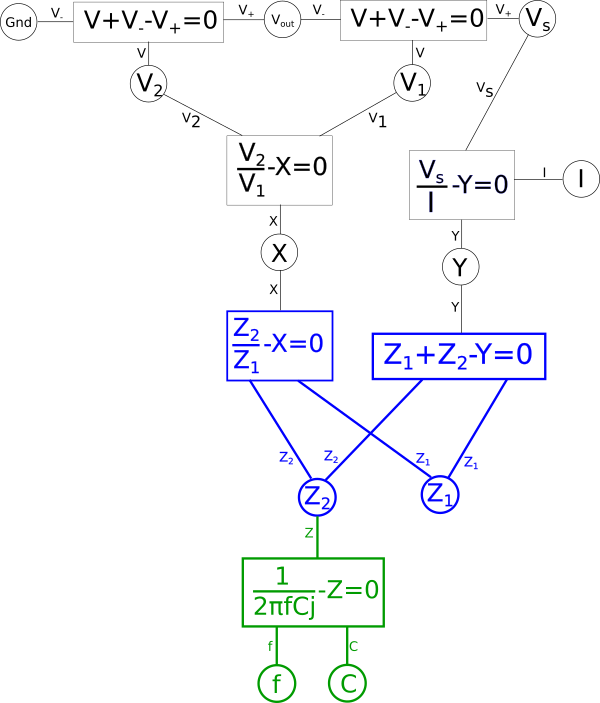
We also want to split the equation on the right hand side for the same reason.
$$ \color{current}\frac{V_s}{Z_1+Z_2}\color{normal} - \color{current}I\color{normal} = 0 $$
$$ \color{current}\frac{V_s}{Z_1+Z_2}\color{normal} = \color{current}I\color{normal} $$
$$ \color{impedance}\frac{1}{Z_1+Z_2}\color{normal} = \color{impedance}\frac{I}{V_s}\color{normal} $$
$$ \color{impedance}Z_1\color{normal} + \color{impedance}Z_2\color{normal} = \color{impedance}\frac{V_s}{I}\color{normal} $$
$$ \color{impedance}Z_1\color{normal} + \color{impedance}Z_2\color{normal} - \color{impedance}\frac{V_s}{I}\color{normal} = 0 $$
Which we can split into our two new equations.
$$ \color{impedance}Z_1\color{normal} + \color{impedance}Z_2\color{normal} - Y = 0 $$
$$ \color{impedance}\frac{V_s}{I}\color{normal} - Y = 0 $$
Representing that in the diagram we get.
We should now take a moment to consider what properties the dual circuit we want to create needs to have in order for it to meet our use case. For the sake of simplicity let's start by saying we don't care about the phase of the AC signals throughout the circuit, only the amplitude. This lets us get rid of the imaginary{: style="color: rgb(251,0,29)"} number, \(\color{imaginary}j\color{normal}\), in our equation for capacitor impedance{: style="color: rgb(18, 110, 213)"} and lets us treat all the variables throughout our system of equations as real numbers. We could handle the complex case if we wanted but for now I think it's important we keep this example simple.
Since we've done away with imaginary{: style="color: rgb(251,0,29)"} and complex numbers let's consider what shared variables in our system of equations need to remain fixed points when we transform it to our dual and what variables are free to change. Keep in mind all the variables in the end will always be a dual of their counterpart in the original, we just decide which variables are fixed points, and thus their own dual, and which are not fixed. Remember an element in a system can always be a dual of itself so this isn't a problem.
Well, \(\color{voltage}V_s\color{normal}\) represents our input signal and \(\color{voltage}Gnd\color{normal}\) defines the bias, or in this case lack of a bias, applied to that signal, so we know those values must be fixed. Similarly we know we want our dual circuit to behave as an equivalent low-pass filter to the original therefore we can also assert that \(\color{voltage}V_{out}\color{normal}\) must likewise be fixed. The rest of the variables we aren't too concerned with, so let's start by coloring our fixed points red.
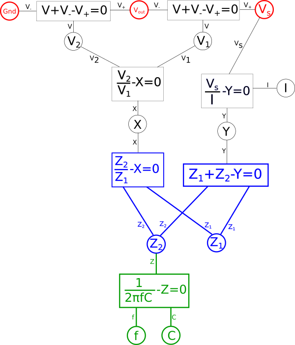
By defining a certain point as fixed this will cause this effect to propagate throughout a portion of our diagram. Essentially any variables in our diagram which are dependent solely on other fixed variables will themselves become fixed variables. To illustrate this first find any equations where either all but one variable directly connected to it is red, or where all variables are red, and make that equation red. Likewise after doing that any equation which is red which connects to a black variable, make that variable red. Repeat this until there are no more changes to be made. Note that at no point will you change the color of anything that is in blue in the diagram.
At this point we have defined our expectations and appropriately annotated our diagram. Everything in red represents the portion of the system that will remain fixed while the black portion will be free to transform. It is important to note that not all choices for fixed points are possible or useful, for example in this case if we had also defined current{: style="color: rgb(0, 255, 221)"}, \(\color{current}I\color{normal}\), as a fixed point then there would be no valid transformation that would satisfy this, we will see why in a moment.
In our diagram any blue equations connected with a red portion will be the equation that will dictate the transform we must use when flipping the green portion of our graph to the other shared variable. If both of the blue equations were connected to a red variable then that would mean that we must satisfy the transform, which we will calculate in a minute, to satisfy both of these equations simultaneously. Often that is not possible, it would only be possible if both equations would somehow dictate the same transform. As we will see in a minute that is not the case here so we know that only one of the two blue equations is allowed to be connected to a red segment. As such we also know that given the fixed points we already selected, annotated in red, it is not possible to also make \(\color{current}I\color{normal}\) fixed. With that said if all we really cared about was \(\color{current}I\color{normal}\) and \(\color{voltage}V_s\color{normal}\) remaining fixed, and allowed the other variables to transform, then that would be doable as well. But if we did that we would be solving a very different problem since we are trying to create a dual which is feature-preserving with regards to still being low-pass filter.
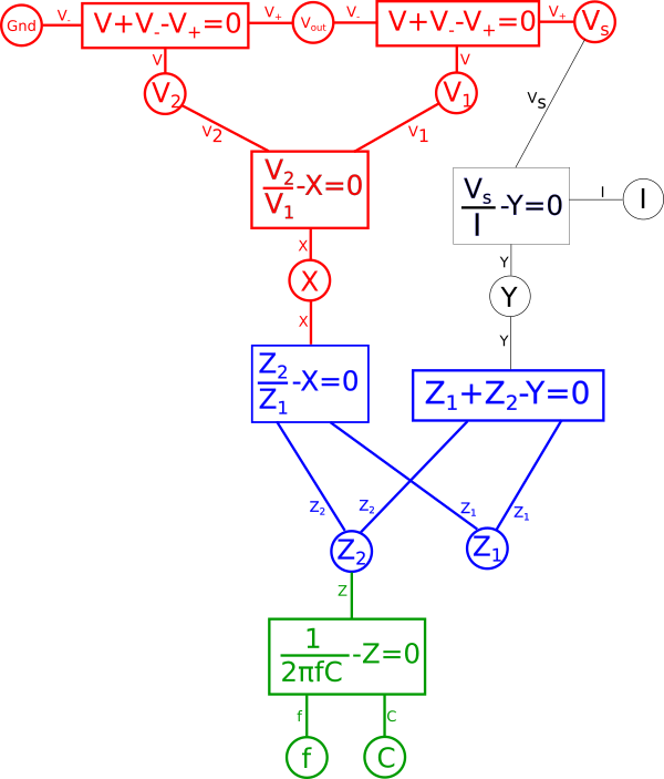
The final step is to figure out the transformation the left-hand blue equation will dictate for a flip across \(\color{impedance}Z_2\color{normal}\) and \(\color{impedance}Z_1\color{normal}\). To do that pick for one of the shared variables at either end and solve for it. In this case we will start with \(\color{impedance}Z_1\color{normal}\).
$$ \color{impedance}Z_2\color{normal} = X \cdot \color{impedance}Z_1\color{normal} $$
$$ \color{impedance}Z_2\color{normal} = X \cdot \color{impedance}Z_1\color{normal} $$
$$ \color{impedance}Z_1\color{normal} = \color{impedance}Z_2\color{normal} \cdot \frac{1}{X} $$
Now solve for the other variable, in this case \(\color{impedance}Z_2\color{normal}\)
$$ \frac{\color{impedance}Z_2\color{normal}}{\color{impedance}Z_1\color{normal}} - X = 0 $$
$$ \frac{\color{impedance}Z_2\color{normal}}{\color{impedance}Z_1\color{normal}} = X $$
$$ \color{impedance}Z_2\color{normal} = X \cdot \color{impedance}Z_1\color{normal} $$
These two equations represent inverses of each other, obviously. Next lets represent them as functions of \(X\) and also make \(\color{impedance}Z_1\color{normal}\) and \(\color{impedance}Z_2\color{normal}\) the same variable as follows.
$$ \color{impedance}Z_1(X)\color{normal} = \frac{1}{X} \cdot \color{impedance}Z\color{normal} $$
$$ \color{impedance}Z_2(X)\color{normal} = X \cdot \color{impedance}Z\color{normal} $$
Next we want to figure out what transformation we have to do to X in one function in order to produce the other function. In other words, we want to figure out what the function \(T(x)\) needs to be in the following equation.
$$ \color{impedance}Z_1(T(X))\color{normal} = \color{impedance}Z_2(X)\color{normal} \label{argtrans} $$
Since the equation here is simple it is probably already obvious, but let's expand our functions and work through it anyway; expanding our two functions for equation \(\eqref{argtrans}\) and we get.
$$ \color{impedance}Z\color{normal} \cdot \frac{1}{T(X)} = X \cdot \color{impedance}Z\color{normal} $$
Let's just solve for \(T(X)\) to see what the function definition is.
$$ \frac{1}{T(X)} = \frac{X \cdot \color{normal}Z\color{impedance}}{\color{impedance}Z\color{normal}} $$
$$ \frac{1}{T(X)} = X $$
$$ T(X) = \frac{1}{X} $$
We also need to find the inverse function of \(T(X)\) which would be the function that satisfies the following.
$$ f^{-1}(T^{-1}(X)) = f(X) $$
Another way of stating the same thing is you just take the function \(T(X)\) and solve for X.
$$ T(X) = \frac{1}{X} $$
$$ y = \frac{1}{X} $$
$$ x = \frac{1}{y} $$
$$ T^{-1}(X) = \frac{1}{X} $$
As we can see in this case the inverse of \T(X)\) is itself. This isnt always the case, as we discussed earlier this makes the transform in this case an involution.
Now we know in order to perform the flip between the two components in the circuit we must perform the reciprocal transform on each component when we do. To do this we can flip the two nodes and insert our reciprocal transformation between each of them. If the transform were not an involution then we would perform the inverse transform on \(\color{impedance}Z_2\color{normal}\) to get \(\color{impedance}Z_{\hat{1}}\color{normal}\) and vice versa as follows.
$$ \color{impedance}Z_{\bar{1}}\color{normal} = T^{-1}(\color{impedance}Z_2\color{normal}) $$
$$ \color{impedance}Z_{\bar{2}}\color{normal} = T(\color{impedance}Z_1\color{normal}) $$
If we were talking about a simple voltage{: style="color: rgb(181, 181, 98)"} divider made with two resistors, where \(\color{impedance}Z_1\color{normal} = \color{resistance}100\Omega\color{normal}\) and \(\color{impedance}Z_2\color{normal} = \color{resistance}10\Omega\color{normal}\), then we could flip the position of these components, take the reciprocal of each and we would have an equivalent system, where \(\color{impedance}Z_{\bar{1}}\color{normal} = \color{resistance}\frac{1}{10}\Omega\color{normal}\) and \(\color{impedance}Z_{\bar{2}}\color{normal} = \color{resistance}\frac{1}{100}\Omega\color{normal}\), and in doing so all other variables in red will remain fixed. Meanwhile, as expected, current{: style="color: rgb(0, 255, 221)"}, \(\color{current}I\color{normal}\), will change significantly. However in this case we are working with a capacitor and a resistor and not two resistors so that changes things. Let's illustrate our new diagram under the transform.
![]()
Lets expand the transform function and we get the following.
![]()
We quickly notice that if we combine the reciprocal equation and the impedance{: style="color: rgb(18, 110, 213)"} equation for the capacitor, it would take the reciprocal and thus eliminate the fraction. What we wind up with looks identical at that point to the equation for an inductor. That is because the impedance{: style="color: rgb(18, 110, 213)"} for an inductor is always the dual of the impedance{: style="color: rgb(18, 110, 213)"} of a capacitor of the same value under the reciprocal transform. As such our capacitor becomes an inductor, therefore we can combine these two equations in our diagram and arrive at the equation for an inductor by changing the variable \(\color{capacitance}C\color{normal}\) to \(\color{inductance}L\color{normal}\), which is convention for representing inductance{: style="color: rgb(255,0,255)"}. Similarly the dual of a resistor's impedance{: style="color: rgb(18, 110, 213)"} under the reciprocal transform would be admittance, which is just the reciprocal of resistance{: style="color: rgb(114,0,172)"}. Therefore we can likewise change the resistor in our original circuit with a new resistor where the capacitor used to be that has an admittance value that is the same as the resistance{: style="color: rgb(114,0,172)"} value of the old resistor. The standard variable for admittance is \(Y\) so lets likewise make that change in our diagram.
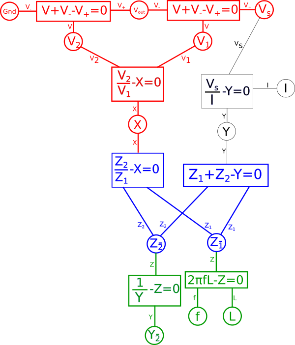
This final diagram is our dual where \(\color{capacitance}C\color{normal} = \color{inductance}L\color{normal}\) in the original circuit and \(Y_{\bar{2}} = \color{inductance}Z_2\color{normal}\) as well. This now represents an inductor based low-pass filter as we illustrated in the circuit diagram earlier.
To recap, we know that the impedance{: style="color: rgb(18, 110, 213)"} equation for an inductor is the reciprocal of that of a capacitor, so in our capacitor based low-pass filter we know we can swap the position of the capacitor and the resistor, use the reciprocal value for the new resistor, and since an inductor is already the reciprocal of a capacitor, we just ensure the inductor has the same inductance{: style="color: rgb(255,0,255)"} in Henrys as the capacitor has capacitance{: style="color: rgb(255, 127, 0)"} in Farads. Thus transforming our capacitor based low-pass filter into its inductor based dual.
The Voltage-current Dual Under Parallel-series Transformation
A voltage{: style="color: rgb(181, 181, 98)"}-current{: style="color: rgb(0, 255, 221)"} circuit dual under parallel-series transformation is another valid type of dual. In this sort of dual points in the circuit that represent voltage{: style="color: rgb(181, 181, 98)"} signals are transformed into equivalent current{: style="color: rgb(0, 255, 221)"} signals and vice versa. Every point in the original circuit that represents a voltage{: style="color: rgb(181, 181, 98)"} has an equivalent current{: style="color: rgb(0, 255, 221)"} through a mesh in the dual circuit. As such the number of nodes in the original circuit (not counting ground) is equal to the number of meshes in the dual circuit and vice versa. This is accomplished by transforming each component from its series topology to a parallel topology and vice versa.
The process for working with the system of equations that define this type of dual is similar to the process we used earlier except we are simply flipping around different parts of the graph and choosing different relationships. I encourage you to give it a try for yourself.
Under this type of dual a voltage{: style="color: rgb(181, 181, 98)"} divider becomes its equivalent, a current{: style="color: rgb(0, 255, 221)"} divider. Take the following voltage{: style="color: rgb(181, 181, 98)"} divider as an example.
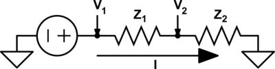
Likewise here is its voltage{: style="color: rgb(181, 181, 98)"}-current{: style="color: rgb(0, 255, 221)"} dual under parallel-series transformation, a current divider.
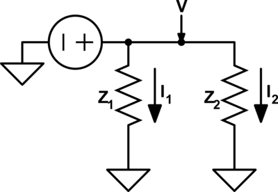
As you can see \(\color{current}I_1\color{normal}\) becomes equivalent to \(\color{voltage}V_1\color{normal}\) and \(\color{current}I_2\color{normal}\) becomes equivalent to \(\color{voltage}V_2\color{normal}\). We can also see that the second circuit has two meshes and one node; meanwhile, the first circuit has two nodes and one mesh. More importantly, however, the ratio of the current{: style="color: rgb(0, 255, 221)"} being divided between \(\color{current}I_1\color{normal}\) and \(\color{current}I_2\color{normal}\) in the current{: style="color: rgb(0, 255, 221)"} divider is the same as the ratio between voltages \(\color{voltage}V_1\color{normal}\) and \(\color{voltage}V_2\color{normal}\) in the voltage{: style="color: rgb(181, 181, 98)"} divider.
The Electric-magnetic Dual under Capacitance-permeance Transformation
There is another type of circuit dual that is far more obscure, rarely understood, and almost never considered, that is the circuit dual created by swapping the magnetic field and the electric field in much the same way we can create a circuit dual that swaps the voltage{: style="color: rgb(181, 181, 98)"} and current{: style="color: rgb(0, 255, 221)"} values. Every electric circuit has an equivalent magnetic circuit as its dual, though in practice this isnt always all that useful to create such a dual. In a magnetic circuit dual of an electric circuit resistance{: style="color: rgb(114,0,172)"} becomes magnetic resistance{: style="color: rgb(114,0,172)"}, electric fields are replaced with magnetic fields, inductors behave like capacitors, capacitors behave like inductors, Electromotive Force (EMF), measured in volts{: style="color: rgb(181, 181, 98)"}, is replaced with Magnetomotive Force (MMF), measured in amps, and current{: style="color: rgb(0, 255, 221)"} is replaced with magnetic current{: style="color: rgb(0, 255, 221)"} which is the rate of change of magnetic flux, which conveniently enough has the units of volts. In other words a magnet or inductor where the field is collapsing or growing at a constant rate in a magnetic circuit is equivalent to a DC an electric circuit. Similarly since a spinning magnet by definition is constantly accelerating at the edges where its two poles are located (remember rotating objects are constantly accelerating at their edge by definition) would be equivalent to an AC electric citcuit.
Resistance{: style="color: rgb(114,0,172)"} is the property of a material to impede the flow of current{: style="color: rgb(0, 255, 221)"} and reluctance is the property of a material to impede the propagation of a magnetic field. Magnetic resistance{: style="color: rgb(114,0,172)"} is closely related to reluctance, at least when represented as a complex number which we will calculate later on. Low reluctance, coupled with high electrical resistivity, gives us low magnetic resistance{: style="color: rgb(114,0,172)"}, however reluctance is a complex value and varies with frequency. Since energy isn't dissipated when a static magnetic field is applied, and thus a static magnetic field does not represent current flow in a magnetic circuit. When a changing magnetic field is applied magnetic resistance{: style="color: rgb(114,0,172)"} does dissipate energy fom magnetic field, so it is functionally equivalent with regard to its ability to do work just as a resistor would be in an electrical circuit. Because of this distinction even copper wires which tend to have relatively low resistance{: style="color: rgb(114,0,172)"} but high reluctance would need to be replaced with iron wires that have a higher electrical resistance{: style="color: rgb(114,0,172)"} but a very low reluctance. So in the end the dual of an electric circuit creates a magnetic circuit that really doesn't look much like what we think of as a circuit at all, but functionally, and in terms of its ability to do work, it will be equivalent.
Even though in a magnetic circuit the units for voltage{: style="color: rgb(181, 181, 98)"} and current{: style="color: rgb(0, 255, 221)"} get swapped this is very different than the voltage{: style="color: rgb(181, 181, 98)"}-current{: style="color: rgb(0, 255, 221)"} dual under parallel-series transformation. In this case we aren't actually swapping the arrangement of components but rather voltage{: style="color: rgb(181, 181, 98)"} and current{: style="color: rgb(0, 255, 221)"} become swapped in place and are represented by entirely different forces, namely those caused by the magnetic field. In doing so the transform is no longer a Series-parallel, the transform is called the capacitance-permeance transform, which we will explain later on.
Keep in mind there are actually two types of magnetic duals, both of which are refered to as a magnetic circuit, and they tend to be a bit different. The type we are describing here is an equivalent-work dual in the sense that if you have an electric circuit that does work, then its magnetic dual as described here will also be doing the same amount of work. This is called the gyrator-capacitor model or less commonly the capacitor-permeance{: style="color: rgb(255, 127, 0)"} model for a magnetic circuit. There is another type of magnetic circuit dual which is more often described but does not preserve work-equivalence, that is called the resistance{: style="color: rgb(114,0,172)"}-reluctance model.
Equivalence
First let's start with an illustration to show how in a magnetic circuit the magnetic field can propagate through an iron wire in much the same way an electric field propagates through a copper wire.
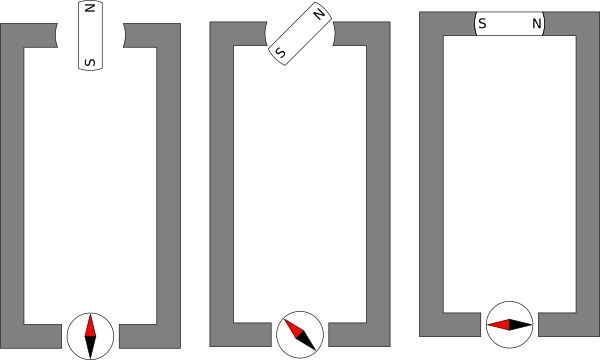
Here we see a permanent bar magnet at the top of each segment and a compass at the bottom. Assume that the distance between the bar magnetic at the top and the compass at the bottom is significant such that the without the iron wire to propagate the magnetic field around the outside, then the bar magnet would have no effect on the compass. We see that by adding the iron wire to propagate the magnetic field we can produce a similar magnetic field at the far end where the compass is at.
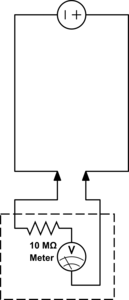
Now in this image the bar magnet in each frame is intended to illustrate a stationary magnet. As such under ordinary conditions the magnet can not do any actual work, the compass will remain in its fixed position. This would be similar to an ordinary electric circuit with a voltage{: style="color: rgb(181, 181, 98)"} applied and no current{: style="color: rgb(0, 255, 221)"} flowing, with a volt{: style="color: rgb(181, 181, 98)"} meter attached in place of the compass. This is not intended to represent the circuit dual of the above but only a demonstration of how magnetic flux propagates through a magnetic conductor in much the same way electric fields propagate through an electric wire.
Before we show actual examples of circuit duals lets cover some of the relevant properties of an electric circuit and their dual in a magnetic circuit.
| Magnetic | Electric | |||||
|---|---|---|---|---|---|---|
| Name | Symbol | Units | Name | Symbol | Units | |
| Magnetomotive force (MMF) | \(\color{voltage}\mathcal{F}\color{normal} = \color{voltage}\int \mathbf{H}\cdot\operatorname{d}\mathbf{l}\color{normal} \) | ampere | Electromotive force (EMF) | \( \color{voltage}V\color{normal} = \color{voltage}\int \mathbf{E}\cdot\operatorname{d}\mathbf{l}\color{normal} \) | volt | |
| Magnetic field | H | ampere/meter = newton/weber | Electric field | E | volt/meter = newton/coulomb | |
| Magnetic flux | \(\Phi\) | weber | Electric charge | Q | Coulomb | |
| Magnetic Current | \( \color{current}\dot \Phi\color{normal} = \color{current}\frac{d\Phi}{dt}\color{normal} \) | weber/second = volt | Current | \( \color{current}I\color{normal} \) | coulomb/second = ampere | |
| Magnetic impedance | \( \color{impedance}\mathcal{Z}(\omega)\color{normal} = \color{impedance}\frac{\mathcal{F}(\omega)}{\dot \Phi(\omega)}\color{normal} \) | 1/ohm = mho = siemens | Impedance | \( \color{impedance}Z(\omega)\color{normal} = \color{impedance}\frac{V(\omega)}{I(\omega)}\color{normal} \) | ohm | |
| Magnetic resistance | \( \color{resistance}\mathcal{R}\color{normal} = \color{resistance}\operatorname{Re}(\mathcal{Z}(\omega))\color{normal} \) | 1/ohm = mho = siemens | Resistance | \( \color{resistance}R\color{normal} = \color{resistance}\operatorname{Re}(Z(\omega))\color{normal} \) | ohm | |
| Magnetic reactance | \( \color{reactance}\mathcal{X}\color{normal} = \color{reactance}\operatorname{Im}(\mathcal{Z}(\omega))\color{normal} \) | 1/ohm = mho = siemens | Reactance | \( \color{reactance}X\color{normal} = \color{reactance}\operatorname{Im}(Z(\omega))\color{normal} \) | ohm | |
| Magnetic admittance | \( \mathcal {Y}(\omega)=\frac{\color{current}\dot \Phi(\omega)\color{normal}}{\color{voltage}\mathcal{F}(\omega)\color{normal}}\) | ohm | Admittance | \( Y(\omega)=\frac{\color{current}I(\omega)\color{normal}}{\color{voltage}\mathcal{E}(\omega)\color{normal}} \) | 1/ohm = mho = siemens | |
| Magnetic conductance | \( \mathcal{G} = \operatorname{Re}(\mathcal{Y}(\omega)) \) | ohm | Electric conductance | \( G = \operatorname{Re}(Y(\omega)) \) | 1/ohm = mho = siemens | |
| Magnetic susceptance | \( \mathcal{B} = \operatorname{Im}(\mathcal{Y}(\omega)) \) | ohm | Electric susceptance | \( B = \operatorname{Im}(Y(\omega)) \) | 1/ohm = mho = siemens | |
| Magnetic inductance | \( \color{inductance}\mathcal{L}\color{normal} = \color{inductance}\frac{\mathcal{X}(\omega)}{\omega}\color{normal} \) | Farad | Inductance | \( \color{inductance}L\color{normal} = \color{inductance}\frac{X(\omega)}{\omega}\color{normal} \) | Henry | |
| Permeance / magnetic capacitance | \( \color{capacitance}\mathcal{C}\color{normal} = \color{capacitance}\frac{\mathcal{B}(\omega)}{\omega}\color{normal} \) | Henry | Capacitance | \( \color{capacitance}C\color{normal} = \color{capacitance}\frac{B(\omega)}{\omega}\color{normal} \) | Farad | |
| Power | \( P = \color{voltage}\mathcal{F}\color{normal} \cdot \color{current}\bar{\dot \Phi}\color{normal} \) | Watts = Joule/second | Power | \( P = \color{voltage}V\color{normal} \cdot \color{current}\bar{I}\color{normal} \) | Watts = Joule/second | |
Ohms law also has its dual for use in a magnetic circuit and it is called Hopkinson's law and is defined in a similar way as Ohm's law except by simply substituting our duals for each property as noted in the above table1.
$$ \color{voltage}\mathcal{F}\color{normal} = \color{current}\frac{d \Phi}{dt}\color{normal} \cdot \color{impedance}\mathcal{Z}\color{normal} $$
Which is sometimes simplified to just the following.
$$ \color{voltage}\mathcal{F}\color{normal} = \color{current}{\dot \Phi}\color{normal} \cdot \color{impedance}\mathcal{Z}\color{normal} $$
Where
\(\color{voltage}\mathcal{F}\color{normal}\) is the magnetomotive force, also called magnetic voltage{: style="color: rgb(181, 181, 98)"}, and is in ampere,
\(\color{current}\frac{d \Phi}{dt}\color{normal}\) or \(\color{current}{\dot \Phi}\color{normal}\) is the rate of change of the magnetic flux also called the magnetic current{: style="color: rgb(0, 255, 221)"}, measured in volts, and
\(\color{impedance}\mathcal{Z}\color{normal}\) is the magnetic impedance{: style="color: rgb(18, 110, 213)"}, which is measured in siemens, the reciprocal unit of the ohm.
As long as these equivalences are kept in mind then we can easily calculate the power of our magnetic circuit in the same way we would an electric circuit. Since this model is work-equivalent a magnetic circuit which is the dual of an electric circuit will always have the same power per component, at least when we represent the components as ideal components. Since power is a measure of the rate at which work is being done we likewise will always have the same work being done by these two circuit duals. This is defined by Joule's Law which in a magnetic circuit is as follows1.
$$ P = \color{voltage}\mathcal{F}\color{normal} \cdot \bar{\color{current}\dot \Phi\color{normal}} $$
Where
\(P\) is the power in watts,
\(\color{voltage}\mathcal{F}\color{normal}\) is the MMF{: style="color: rgb(181, 181, 98)"}. in ampere, and
\(\bar{\color{current}\dot \Phi\color{normal}}\) is the conjugate of the magnetic current{: style="color: rgb(0, 255, 221)"}, in volts.
Of course you only need to take the conjugate when dealing with complex numbers in the frequency domain, in the time domain where we use real numbers the conjugate of a real number is always itself, so this can be ignored. Keep in mind in the frequency domain these values must be in RMS form and not absolute magnitudes.
One other minor consideration here is that a magnetic dual circuit will have magnetic field lines that are perpendicular to the orientation of magnetic fields in its electric dual. Similarly the magnetic field lines in the magnetic circuit will be parallel to the electric field lines in the electric circuit. For example the magnetic field lines which surround the wires in a magnetic circuit run parallel and along the wires unlike in an electric circuit where they form concentric circles around the wires.
Magnetic DC and AC Current
When we talk about magnetic DC or AC current{: style="color: rgb(0, 255, 221)"} things get a bit confusing. In practice most authors would simply avoid these terms all together, and for good reason. But as should be obvious at this point every concept in our electric circuit model has a dual in the magnetic circuit model, so it is worth touching on this.
The reason it is a bit misleading is because in an electric circuit a DC current{: style="color: rgb(0, 255, 221)"} implies electrons are moving in a single direction at a constant rate, the electrons never speed up or slow down. However remember that in a magnetic circuit current{: style="color: rgb(0, 255, 221)"} is defined as the rate of change of flux, \(\color{current}\dot{\Phi}\color{normal} = \color{current}\frac{d\Phi}{dt}\color{normal}\). This means the dual of a DC current{: style="color: rgb(0, 255, 221)"} from an electric circuit would be a constantly increasing (or decreasing) flux, \(\Phi\), in a magnetic circuit. Such an effect could be produced if the source of the magnetic field feeding into our magnetic circuit happened to be an ideal voltage{: style="color: rgb(181, 181, 98)"} source connected to an ideal inductor. As you know as an inductor decreases its impedance{: style="color: rgb(18, 110, 213)"} in the time-domain as it charges, therefore in order to maintain a constant voltage{: style="color: rgb(181, 181, 98)"} across an inductor the current{: style="color: rgb(0, 255, 221)"} through the inductor would have to increase at a constant rate, thus resulting in a constant rate of increase in the magnetic flux it produces.
While in a theoretical context where we are modeling a magnetic circuit with ideal components this sense of a DC circuit works just fine. However in the real world parasitic resistance{: style="color: rgb(114,0,172)"} would quickly overwhelm the ever increasing current{: style="color: rgb(0, 255, 221)"} and make any magnetic DC current{: style="color: rgb(0, 255, 221)"} that is sustained for an appreciable length of time impractical. So while we can talk about magnetic DC currents{: style="color: rgb(0, 255, 221)"} as a way of better understanding the duality, in practice, they're not something we are likely to employ for any length of time as we we would with DC in an electric circuit.
On the other hand AC magnetic circuits are perfectly fine and in fact the norm. If the same voltage{: style="color: rgb(181, 181, 98)"} source combined with an inductor was used as the power source but the voltage{: style="color: rgb(181, 181, 98)"} source was made into a sinusoidal AC voltage{: style="color: rgb(181, 181, 98)"} instead then the resulting changing magnetic flux would represent an AC magnetic circuit. This would also be equivalent to a rotating magnet with a constant angular velocity in place of the inductor and voltage{: style="color: rgb(181, 181, 98)"} source.
The Magnetic Capacitor
Much as an electric capacitor is a component which acts as a reservoir able to to store energy in the form of an electric field or convert that stored energy back into current{: style="color: rgb(0, 255, 221)"} in an electric circuit, a magnetic capacitor is a component of a magnetic circuit that acts as a reservoir for energy in the form of a magnetic field. Similarly an electric capacitor is made of two electrically conductive plates with a material in between them which has high permittivity{: style="color: rgb(255,0,0)"} and high resistance{: style="color: rgb(114,0,172)"} a good magnetic capacitor would consist of two plates made of material with high magnetic conductivity with a material between them which has high permeability{: style="color: rgb(0,255,0)"} and a low magnetic resistance{: style="color: rgb(114,0,172)"}, which we will cover in the next section. Remember as we pointed out in our table of duals above, permeability{: style="color: rgb(0,255,0)"} is to the magnetic field what permittivity{: style="color: rgb(255,0,0)"} is to the electric field, and electric resistance{: style="color: rgb(114,0,172)"} has the reciprocal units of magnetic resistance{: style="color: rgb(114,0,172)"}. We cover the relationship between electrical resistance{: style="color: rgb(114,0,172)"} and magnetic resistance{: style="color: rgb(114,0,172)"} in more detail in the next section but for now just keep in mind that higher electrical resistance{: style="color: rgb(114,0,172)"} of a material results in lower magnetic resistance{: style="color: rgb(114,0,172)"} for that same material. As such a good magnetic capacitor will usually be made of a material with high electrical resistance{: style="color: rgb(114,0,172)"}.
In practice since the wires that connect the components in a magnetic circuit tend to have low magnetic resistance{: style="color: rgb(114,0,172)"} by design, usually made of iron ferrite, it is typical that the plates of a magnetic capacitor are made of the same material as that which is filling the space between the plates, where you would normally expect a dielectric to be in an electric capacitor. As such a magnetic capacitor is nothing more than a block of material usually of the same construction as your magnetic wires, and there are effectively no actual plates of any kind, just the surface at each end of the block. None the less the surface area of the plane at each end of the block of material determines the magnetic capacitance{: style="color: rgb(255, 127, 0)"} in much the same way the surface area of the plates in an electric capacitor would, that is, the larger the surface area the greater the capacitance{: style="color: rgb(255, 127, 0)"} in both the electric and magnetic duals of a capacitor. Similarly in much the same way the distance between the two plates lowers the capacitance{: style="color: rgb(255, 127, 0)"} in an electric capacitor, the length of the block of material making up our magnetic capacitor also lowers the magnetic capacitance{: style="color: rgb(255, 127, 0)"} of our magnetic capacitor.
This contrast may seem odd at first but when you think about it a bit further it actually makes a lot of sense. In an electric circuit an inductor is really just a long wire, we tend to coil them up to save some space or help direct the magnetic field, but a copper wire is just an inductor. The only real difference between an inductor and a wire is the geometry, and the specific geometry or a wire, particularly if it is very long, along with the frequency traveling through it, determines if the inductive effects are significant or not. In electric circuits when an ordinary wire happens to be long enough where the inductive effects become significant we would call that parasitic inductance{: style="color: rgb(255,0,255)"}. Likewise if a magnetic wire has dimensions that are sufficient to cause it to have a significant and unwanted magnetic capacitance that would simply be parasitic capacitance{: style="color: rgb(255, 127, 0)"} for a magnetic circuit. So its really not that odd at all that every magnetic wire is effectively a magnetic capacitor since in the electric domain every electric wire is effectively an inductor.
The fact that a magnetic capacitor is just a block of iron or iron ferrite actually makes a lot of sense when you think about it, afterall in a ferrite core inductor the core's purpose is to act as a reservoir to hold the magnetic field in a smaller space than what would be needed for an air core. So even in an electric circuit iron ferrite acts as a magnetic field reservoir.
Note that magnetic capacitance{: style="color: rgb(255, 127, 0)"} is just another word for permeance{: style="color: rgb(255, 127, 0)"}, the two terms can be used interchangeably. Likewise permeance{: style="color: rgb(255, 127, 0)"} is also simply the reciprocal of reluctance. Usually when modeling capacitors in either an electric circuit or magnetic circuit we treat the capacitors as ideal components that experience no resistive loss; resistive loss in a capacitor is called ESR, effective series resistance{: style="color: rgb(114,0,172)"}. However in the real world if we wish to model a real electrical or magnetic capacitor we must measure their respective capacitance{: style="color: rgb(255, 127, 0)"} as complex values instead, which enables us to calculate the ESR. For the same reason we also use complex permittivity{: style="color: rgb(255,0,0)"} or complex permeability{: style="color: rgb(0,255,0)"} when calculating the capacitance{: style="color: rgb(255, 127, 0)"}/permeance{: style="color: rgb(255, 127, 0)"} for the same reason, at least when we aren't dealing with an ideal model. We cover all this in more detail in the section on magnetic resistance{: style="color: rgb(114,0,172)"}, but for now just keep in mind magnetic capacitance{: style="color: rgb(255, 127, 0)"} can be represented as a complex value if we wish to determine the ESR. Many of you who are used to doing models of electric circuits likely only ever considered capacitors as ideal components and thus are only familiar with real number values for capacitance{: style="color: rgb(255, 127, 0)"}; the same ideal model approach can be used here. If considering a magnetic capacitor as ideal then it is usually acceptable to simply represent its capacitance{: style="color: rgb(255, 127, 0)"} as a real number as we would with analysis of electric circuits.
The following is the equation for determining the complex magnetic capacitance{: style="color: rgb(255, 127, 0)"} of a component2.
$$ \color{capacitance}\mathcal{C}{{real}}\color{normal} = \color{capacitance}\mu\cdot\frac{S}{L}\color{normal} \label{realcap}$$
Where
\(\color{capacitance}\mathcal{C}{{real}}\color{normal}\) is the complex magnetic capacitance{: style="color: rgb(255, 127, 0)"}, also called permeance{: style="color: rgb(255, 127, 0)"}, the unit of which is the Henry,
\(\color{permeability}\mu\color{normal}\) is the complex2 permeability{: style="color: rgb(0,255,0)"} of the material at the given frequency,
\(S\) is the cross sectional surface area of the material, and
\(L\) is the length of the material.
If we wish to calculate the real-value magnetic capacitance{: style="color: rgb(255, 127, 0)"} of an idealized capacitor the equation is the same except \(\color{permeability}\mu\color{normal}\) becomes a real number; specifically it looses its real component and only represents the magnitude of the imaginary{: style="color: rgb(251,0,29)"} part of the complex permeability{: style="color: rgb(0,255,0)"}1. The specific equation would then look like the following.
$$ \color{capacitance}\mathcal{C}{{ideal}}\color{normal} = \color{capacitance}\mu'' \frac{S}{L}\color{normal} \label{idealcap}$$
where
\(\color{capacitance}\mathcal{C}{{ideal}}\color{normal}\) is the idealized real-value magnetic capacitance{: style="color: rgb(255, 127, 0)"}, and
\(\mu^{\prime\prime}\) is the imaginary{: style="color: rgb(251,0,29)"} component of the complex2 permeability{: style="color: rgb(0,255,0)"} of the material at the given frequency.
Specifically \(\mu^{\prime\prime}\) relates to the complex permeability{: style="color: rgb(0,255,0)"} as follows.
$$ \color{permeability}\mu\color{normal} = \color{permeability}\mu' - j\mu''\color{normal} $$
The following diagram shows an example demonstrating the above equation for a block of material.
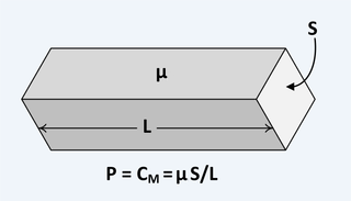
Keep in mind depending on if you use the complex capacitance{: style="color: rgb(255, 127, 0)"} equation above \(\eqref{realcap}\), or the idealized form \(\eqref{idealcap}\), would affect how you construct reactance{: style="color: rgb(45,177,93)"} and impedance{: style="color: rgb(18, 110, 213)"} equations. The ideal form drops the imaginary{: style="color: rgb(251,0,29)"} number and as such is always positive, so when constructing the impedance{: style="color: rgb(18, 110, 213)"} you must explicitly add the imaginary{: style="color: rgb(251,0,29)"} number back in, for example. This is the approach most people are used to since capacitors are usually modeled as ideal. However in the real-world capacitance{: style="color: rgb(255, 127, 0)"} equation the imaginary{: style="color: rgb(251,0,29)"} number is already included in the complex value \(\color{permeability}\mu\color{normal}\) therefore when using that form of the equation to construct your impedance{: style="color: rgb(18, 110, 213)"} values you do not need to add the imaginary{: style="color: rgb(251,0,29)"} number back in, however when using it to construct the reactance{: style="color: rgb(45,177,93)"} value you must make sure to take the imaginary{: style="color: rgb(251,0,29)"} part, which will be negative, and drop the \(\color{imaginary}j\color{normal}\). Whichever approach you use, be sure to be consistent. The following demonstrates this.
$$ \color{impedance}\mathcal{Z}\color{normal} = \frac{1}{\omega\color{capacitance}\mathcal{C_{{ideal}}}\color{imaginary}j\color{normal}} = \frac{1}{\omega\color{capacitance}\mathcal{C{_{real}}}\color{normal}} $$
$$ \color{reactance}\mathcal{X}\color{normal} = -\frac{1}{\omega\color{capacitance}\mathcal{C_{{ideal}}}\color{normal}} = \operatorname{Im}\left(\frac{1}{\omega\color{capacitance}\mathcal{C{_{real}}}\color{normal}}\right) $$
The Magnetic Inductor and Gyrator
As discussed in the previous section in an electric circuit a capacitor is a component which acts as a reservoir for an electric field where it can store energy from the circuit as well as deliver that energy back into the circuit. Similarly in an electric circuit an inductor is a component which acts as a reservoir for a magnetic field which can store or deliver energy from, and to, the circuit. In addition a capacitor in an electrical circuit is storing the type of field, the electric field, being worked within the wires of an electrical circuit, this should be obvious as an electric voltage{: style="color: rgb(181, 181, 98)"} between two points is the measure of the difference in the strength of the electric field between those points, and electric current{: style="color: rgb(0, 255, 221)"} is the movement of electrons, an electric charge carrier. This is why we can measure the voltage{: style="color: rgb(181, 181, 98)"} across a capacitor and use that to indicate how full the capacitor happens to be. Likewise as we recently covered the magnetic capacitor stores a magnetic field instead, which is similarly the type of field inherent to a magnetic circuit. This is contrasted with an electric inductor; in an electric circuit, an inductor stores energy in the form of a magnetic field, which is not the type of field propagating through an electric circuit's copper wires, outside of parasitic effects or inductors anyway, though even in that case the magnetic field largely manifests outside of the copper wires themselves. So in a sense the purpose of an inductor in an electric circuit is to convert the intrinsic electric field energy of the circuit into magnetic field energy, and then store it. In the case of an electric inductor this is stored in the ferrite core, in the case of an air core inductor it is stored in the space around the inductor. This analogy also applies when we talk about magnetic inductors, that is, their purpose is to convert the intrinsic magnetic field energy of a magnetic circuit into electrical field energy and store this energy, or to deliver that stored energy back into the magnetic circuit.
One thing that may be obvious from the description I just gave is that an electric inductor, like its magnetic inductor counterpart, is a component that is capable of converting electric energy into magnetic energy, and its magnetic inductor counterpart must reverse this process and be able convert magnetic energy into electric energy. However we already know that an electric inductor works in both directions; just as the electric energy of the circuit can charge it, converting it to magnetic energy stored in its ferrite core, it can also take that stored magnetic energy in the ferrite core and deliver it back into the circuit in the form of electric energy. In magnetic circuits a component that is able to convert electric energy into magnetic energy, and magnetic energy into electric energy is called a gyrator, and it's really no different than what we think of as an electric inductor already, just working in the opposite direction. Keep in mind a gyrator is not the magnetic dual of an electric inductor, a magnetic inductor, but it is essential in getting there, which we will do in a moment, first let me finish explaining what a gyrator is.
Again, a gyrator is nothing more than an electrical inductor wrapped around a magnetic conductor of some type, usually a ferrite core or a piece of iron. Despite this, because it is viewed a bit differently than we tend to view an inductor used an electric circuit it is given a special name, and even its own circuit symbol. It is best to view a gyrator as a component that converts between electrical and magnetic energy. The following is a diagram that demonstrates this.
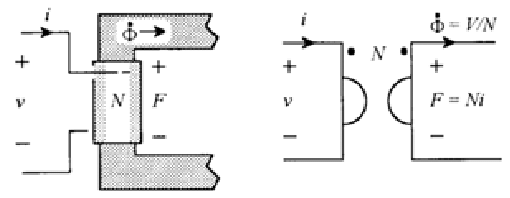
In the above diagram we see the physical gyrator on the left hand side as an inductor wrapping around a ferrite core, with electrical leads protruding to the left, and then the ferrite core becomes the wires of the magnetic circuit. The leads to the magnetic circuit extend to the right of the diagram. On the right hand side of the diagram we see what the schematic symbol for a gyrator looks like in a magnetic circuit schematic.
One interesting point is that your instinct might be to think of the electrical current{: style="color: rgb(0, 255, 221)"} through the inductor as being translated to the magnetic current{: style="color: rgb(0, 255, 221)"} in the core, but in fact that isn't the case. If you recall from our table above relating the duals in a magnetic circuit to those in an electric circuit you can see that the dual for the EMF (Electromotive Force), measured in volts{: style="color: rgb(181, 181, 98)"}, of an electric circuit is the MMF (Magnetomotive Force), measured in ampere13, in a magnetic circuit; likewise the dual for the electric current{: style="color: rgb(0, 255, 221)"}, measured in ampere, is the magnetic current{: style="color: rgb(0, 255, 221)"}, measured in volts{: style="color: rgb(181, 181, 98)"}, and is equivalent to the rate of change of the magnetic flux in the circuit, \(\dot{\Phi}\)34. This may seem odd but it actually makes some sense when you consider the context of a gyrator. Consider Faraday's law which relates the rate of change of the magnetic flux of an inductor with the voltage{: style="color: rgb(181, 181, 98)"} across it.
$$ \color{voltage}V\color{normal} = N \cdot \color{current}\frac{d\Phi}{dt}\color{normal} = N \cdot \color{current}\dot{\Phi}\color{normal}$$
Where
\(\color{voltage}V\color{normal}\) is the EMF{: style="color: rgb(181, 181, 98)"} (Electromotive Force{: style="color: rgb(181, 181, 98)"}) in volts,
\(N\) is the number of turns of the inductor, and
\(\color{current}\frac{d\Phi}{dt}\color{normal}\) and \(\color{current}\dot\Phi\\color{normal}) are the rate of change of the magnetic flux, also called the magnetic current{: style="color: rgb(0, 255, 221)"}, in volts.
It should be clear from this relationship that the magnetic current{: style="color: rgb(0, 255, 221)"}, \(\color{current}\dot\Phi\color{normal}\), is simply the voltage{: style="color: rgb(181, 181, 98)"} across the inductor divided by the number of turns in the inductor.
$$ \color{current}\dot\Phi\color{normal} = \frac{\color{voltage}V\color{normal}}{N}$$
Since \(N\) is a dimensionless unit we can presume that \(\color{current}\dot\Phi\color{normal}\) uses the same units as \(\color{voltage}V\color{normal}\), volts. Similarly the Magnetomotive Force{: style="color: rgb(181, 181, 98)"}, MMF{: style="color: rgb(181, 181, 98)"}, of an inductor is defined as the current{: style="color: rgb(0, 255, 221)"} through the inductor multiplied by the number of turns of the inductor1.
$$ \color{voltage}\mathcal{F}\color{normal} = N \cdot \color{current}I\color{normal} $$
Where
\(\color{voltage}\mathcal{F}\color{normal}\) is the MMF{: style="color: rgb(181, 181, 98)"} (Magnetomotive Force{: style="color: rgb(181, 181, 98)"}) in ampere,
\(N\) is the number of turns of the inductor, and
\(\color{current}I\color{normal}\) is the current{: style="color: rgb(0, 255, 221)"} through the inductor in ampere.
One problem with the standard diagram for a gyrator as shown above is it doesn't actually indicate what side is the electric side housing the leads into the electric inductor, and what side is the magnetic side. This is somewhat intentional as it is intended to be a generic component acting as a blackbox which inverts voltage{: style="color: rgb(181, 181, 98)"} and current{: style="color: rgb(0, 255, 221)"} from wide side onto the inverse on the other. Since in the real world the distinction between the two halves of a gyrator is important lets use the following block diagram for a gyrator instead so I can explicitly illustrate the electric side, on the left in this block diagram, and the magnetic side, on the right.
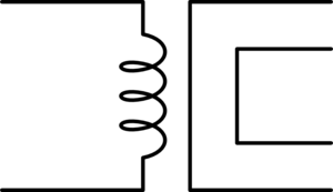
Here is the cool part, if we put two gyrators in series connected by the magnetic side, and optionally adjust the number of turns in the inductor, we have a plain old electric transformer with an iron or iron ferrite core, such as the following.
![]()
Likewise if we connect two gyrators in series but this time connect them on their electric side, again optionally carrying the number of turns, we would have the magnetic circuit dual of a transformer.
![]()
So by now you might be wondering how all this ties into the magnetic circuit dual of an inductor, the magnetic inductor. Well as described in the introduction to this section a magnetic inductor is a component that converts the magnetic energy in a magnetic circuit into an electric field and stores it, and is able to deliver that energy back into the circuit. To do that we simply use a gyrator to convert the magnetic energy into electric, and then use an electric capacitor hooked up to the leads in order to act as the reservoir for the energy stored as an electric field. The following diagram would illustrate a magnetic inductor.
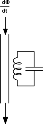
Magnetic Impedance, Resistance, and Reactance
Magnetic resistance{: style="color: rgb(114,0,172)"} is the dual of electrical resistance{: style="color: rgb(114,0,172)"}; just as electrical resistance{: style="color: rgb(114,0,172)"} impedes the flow of electric current{: style="color: rgb(0, 255, 221)"} by converting its energy into heat, magnetic resistance{: style="color: rgb(114,0,172)"} impedes the flow of a changing magnetic field, magnetic current{: style="color: rgb(0, 255, 221)"}, by converting some portion of that energy into heat.
In the resistance{: style="color: rgb(114,0,172)"}-reluctance Model of a magnetic circuit, which is not the model we have been discussing, the dual of resistance{: style="color: rgb(114,0,172)"} is simply reluctance. Reluctance does change with frequency, and can attenuate the propagation of magnetic flux through it. Materiales with high reluctance will show the magnetic flux declining at a greater rate due to distance. However this is not necceseraly due to energy dissipation of the magnetic field itself, particularly when dealing with a static magnetic field, no energy is lost due to reluctance. Reluctance of a material will effect a static magnetic field such as a permanent magnet and not just changing fields. Since it doesn't necceseraly reduce the quantity of energy in the system, then by definition, it is not resistance{: style="color: rgb(114,0,172)"}.
In the model for magnetic circuits we are discussing, the capacitor-permeance{: style="color: rgb(255, 127, 0)"} model, the dual of electrical resistance{: style="color: rgb(114,0,172)"} is called magnetic resistance{: style="color: rgb(114,0,172)"}. Bear in mind that in this particular model both magnetic current{: style="color: rgb(0, 255, 221)"} and magnetic resistance{: style="color: rgb(114,0,172)"} mean something different than in the resistance{: style="color: rgb(114,0,172)"}-reluctance model. In the resistance{: style="color: rgb(114,0,172)"}-reluctance model magnetic current{: style="color: rgb(0, 255, 221)"} is the magnetic field itself, and as such a static field, such as with a permanent magnet, constantly has current{: style="color: rgb(0, 255, 221)"}, and reluctance impedes that current{: style="color: rgb(0, 255, 221)"}. However as mentioned earlier because that model is not work-equivalent to an electric circuit the presence of current{: style="color: rgb(0, 255, 221)"} or resistance{: style="color: rgb(114,0,172)"} in that case does not imply any loss of energy as we normally would think of when we talk about a current{: style="color: rgb(0, 255, 221)"} relative to resistance{: style="color: rgb(114,0,172)"}. This is the reason the resistance{: style="color: rgb(114,0,172)"}-reluctance Model is rarely used, it isn't consistent with the expected meaning of those terms. However in the capacitor-permeance{: style="color: rgb(255, 127, 0)"} model we have been discussing the current{: style="color: rgb(0, 255, 221)"} is not the magnetic field but rather the rate of change of the magnetic field, and resistance{: style="color: rgb(114,0,172)"} is not reluctance but magnetic resistance{: style="color: rgb(114,0,172)"} which is a materials ability to convert a changing magnetic field into heat. This is analogous with dielectric Loss of a capacitor in a changing electric field, which we often see in capacitors and give rise to their ESR, and thus energy loss as heat. In case of magnetic resistance{: style="color: rgb(114,0,172)"} it is the same effect but with regards to the magnetic field instead.
Remember from earlier in the section where we discussed magnetic capacitors that we pointed out that a magnetic capacitor is the same as a magnetic wire, a ferrite core usually, with dimenions sufficient enough for the capacitance{: style="color: rgb(255, 127, 0)"} to be relevant, and like electric capacitors a magnetic capacitor is designed using materials that ensure it has a low magnetic resistance{: style="color: rgb(114,0,172)"}, which implies it will also have a high electrical resistance{: style="color: rgb(114,0,172)"}. So the only real difference between a magnetic capacitor and a magnetic wire is that the material and dimensions of a magnetic wire is selected to minimize both magnetic resistance{: style="color: rgb(114,0,172)"} and magnetic capacitance{: style="color: rgb(255, 127, 0)"}, meanwhile a magnetic capacitor has materials and dimensions selected to minimize magnetic resistance{: style="color: rgb(114,0,172)"} but maximize magnetic capacitance{: style="color: rgb(255, 127, 0)"}. In the same sense a magnetic resistor is no different; it is a block of material representing the component where the materials and dimensions are selected so as to have the magnetic resistance{: style="color: rgb(114,0,172)"} match the intended resistance{: style="color: rgb(114,0,172)"} value while minimizing magnetic capacitance{: style="color: rgb(255, 127, 0)"}. This is not all that different from an electric resistor in the sense that its materials and dimensions are selected to match a particular electrical resistance{: style="color: rgb(114,0,172)"} while minimizing its electrical inductance{: style="color: rgb(255,0,255)"}. This is why we dont use long copper wires for resistors, if the wire is long enough it can have the desired electrical resistance{: style="color: rgb(114,0,172)"} but its inductance{: style="color: rgb(255,0,255)"} would be too high to be useful, so we usually try to design electric resistors to be as short as possible.
Before we can understand magnetic resistance{: style="color: rgb(114,0,172)"} I think its important to understand the analogous concept of electrical resistance{: style="color: rgb(114,0,172)"} of materials and how it arises at various frequencies, especially since most of the time it is grossly oversimplified and misunderstood even in electrical circuits. Contrary to typical thinking electrical resistance{: style="color: rgb(114,0,172)"} isn't simply a static property where materials have inherent resistance{: style="color: rgb(114,0,172)"}, although that can sometimes be the case. A resistor for example always has about the same resistance{: style="color: rgb(114,0,172)"}, sure it varies a little with heat or other conditions, but for the most part the resistance{: style="color: rgb(114,0,172)"} will stay about the same regardless of frequency or other influences. But a resistor is just one very straight forward and simple example of how electrical resistance{: style="color: rgb(114,0,172)"} may present in a circuit. In reality resistance{: style="color: rgb(114,0,172)"} is a much more generalized idea, electrical resistance{: style="color: rgb(114,0,172)"} represents the ability of a material or component to convert current{: style="color: rgb(0, 255, 221)"} into energy that escapes the circuit in some way. In the case of a electical resistor it is converting energy from the electrical current{: style="color: rgb(0, 255, 221)"}, and thus reducing the flow of current{: style="color: rgb(0, 255, 221)"} by doing so, and releasing that energy into the surrounding air in the form of heat. The energy contained in the heat released will be the same quantity of energy as the energy that was removed from the circuit.
When we talk about power in a circuit, more specifically real power, which is the real value component of power when power is represented as a complex number, we are talking about the rate at which a circuit does work. This is another way of saying, in the case of resistors anyway, the rate at which energy in the circuit is converted into heat energy. This definition is the same whether we are talking about magnetic circuits or electric, therefore the real measured resistance{: style="color: rgb(114,0,172)"} of a circuit also means the same between between an electric and magnetic circuit, that is, the ability to convert their respect forms of current{: style="color: rgb(0, 255, 221)"} into heat. Where the difference between these crops up is in the nuance, in realizing that measured real world resistance{: style="color: rgb(114,0,172)"} is not completely determined by circuit resistance{: style="color: rgb(114,0,172)"} due to resistivity. Let me give a real world example of this, again, in the simple to understand electrical circuit model. If you have an antenna and that antenna is well tuned to the frequency of the signal in a circuit it will typically be said to have a 50 ohm impedance{: style="color: rgb(18, 110, 213)"}, this is a real value impedance{: style="color: rgb(18, 110, 213)"}, therefore it is resistance{: style="color: rgb(114,0,172)"}, not reactance{: style="color: rgb(45,177,93)"}. In other words at that particular frequency it is behaving as if it were a physical 50 ohm resistor. The difference is that while a resistor is doing work that causes heat to be produced the antenna is doing work that causes RF waves to be propagated out into space. But in terms of your instruments if you measure the real resistance{: style="color: rgb(114,0,172)"} in the circuit due to the antenna at the given frequency it will have real (not imaginary{: style="color: rgb(251,0,29)"}) resistance{: style="color: rgb(114,0,172)"}, it will look indistinguishable from a resistor; the same energy is being lost at the same rate as in a resistor but simply as RF energy rather than heat. In other words the circuit has real resistance{: style="color: rgb(114,0,172)"} despite the fact that the components itself have 0 resistivity; if you measured resistance using an ohm meter, which measures DC resistance only, it would not be the same. As an important side note, the antenna would be distinguishable, however, from a capacitor or inductor with a 50 ohm impedance{: style="color: rgb(18, 110, 213)"}. In that case the impedance{: style="color: rgb(18, 110, 213)"} of a capacitor or inductor at 50 ohms would be entirely imaginary{: style="color: rgb(251,0,29)"}, not real, and as such would not look at all like the antenna or a resistor in our case; we would call this reactance{: style="color: rgb(45,177,93)"}, not resistance{: style="color: rgb(114,0,172)"}. Because capacitors and inductors have minimal real resistance{: style="color: rgb(114,0,172)"} they don't do any work, no energy is released from the circuit, instead the energy is stored in the capacitor or inductor and usually injected back into the circuit at a later point, which is not at all the same thing.
So now that we understand a bit about the nature of real measured resistance{: style="color: rgb(114,0,172)"} of a circuit at a given frequency is not the same as the resistance{: style="color: rgb(114,0,172)"} of a circuit at DC, or its resistivity, lets try to express how we define that in the electric world using some actual math. This should give us an understanding that we can use to see how this is similar to the same sorts of equations in our magnetic circuit dual. A great example of this in electric circuits is the ESR, equivalent series resistance{: style="color: rgb(114,0,172)"}, that arises when we add a capacitor to a circuit that uses a dielectric material other than a vacuum. Bear in mind a capacitor is very similar to an open circuit where the high resistance{: style="color: rgb(114,0,172)"} is due to a dielectric rather than air. In this case the ESR arises due to two factors, one is the actual real resistance{: style="color: rgb(114,0,172)"} of the material at DC, which tends to be very high, and as such has minimal effect on ESR. The other is due to losses caused by a changing electric field through the dielectric material, it is this part of the real resistance{: style="color: rgb(114,0,172)"} which will vary significantly with frequency and as such the ESR of a capacitor also varies significantly with frequency.
Keep in mind that because in a magnetic circuit wires, capacitors, and resistors are all modeled similarly we will find the equations we go over when talking about electrical capacitors will have direct relevance in describing magnetic resistance{: style="color: rgb(114,0,172)"}, so just bear with me and this will all make sense by the end.
The loss rate of energy in a material at a particular frequency is called the loss tangent it is also called the dissipation factor, it is a unitless ratio and is almost always a positive value. A value of infinity indicates that all the energy it takes from the circuit is lost. For example a resistor has a loss tangent that is extremely large at most frequencies since almost all of the energy it consumes is lost as heat. Likewise a perfectly resonant antenna presenting as 50 ohms real resistance{: style="color: rgb(114,0,172)"} at a given frequency has a similarly extremely large loss tangent at that given frequency; though unlike the resistor the loss tangent will vary as the frequency changes and the antenna is no longer in tune. Similarly an ideal capacitor or inductor, which by definition would have an ESR of 0, has a loss tangent value of 0 because all the energy consumed by the capacitor or inductor is stored in their respective fields and are not lost to the circuit; at a later point in the AC cycle that energy can, and often is, recovered by injecting that energy back into the circuit as the component discharges. In reality most real world components exhibit a finite, non-zero, loss tangent. In addition there are several types of loss tangent, and more generally energy loss, for any any component, at a given frequency, which combine to give the overall loss tangent. For example there is a loss tangent due to the magnetic field, a loss tangent due to the electric field, and energy loss due to resistivity, which can be measured as DC resistance. In some cases, depending on how deep your analysis is going, each of these loss tangents maybe be broken down further into multiple loss tangents that add up as well, but we wont go that deep here. Typically in many real world applications only one of the two types of loss tangent mentioned is dominant or relevant; for example in an electrical capacitor the majority of the loss is due to the dielectric's interaction with the changing electric field, since that is the dominant field passing through the dielectric. Similarly for an electrical inductor it is mostly the magnetic loss that is dominant, and for an electrical resistor it is mostly loss due to resistivity. However even though only one tend to dominate for each component in reality all three do have some effect in order to add up to the total loss tangent.
As mentioned for an electrical capacitor the dominant loss tangent is the electric loss tangent, however even though the loss due to resistivity is minimal it does have an effect, and that effect becomes significant if the dielectric is not a very good resistor. When we analyze a capacitor we usually consider the combined effect of the electric loss tangent and the resistive loss, which is called the dielectric loss tangent. The following is the definition for the dielectric loss tangent5:
$$ \tan{(\delta_d)} = \frac{\omega\varepsilon'' + \sigma}{\omega\varepsilon'} \label{dieleclosstan}$$
Where
\(\omega\) is the angular frequency of the signal,
\(\sigma\) is the DC conductivity of the material, and
\(\varepsilon'\) and \(\varepsilon^{\prime\prime}\) are components of the complex permittivity{: style="color: rgb(255,0,0)"}, \(\color{permittivity}\varepsilon\color{normal}\) of the material such that.
$$ \color{permittivity}\varepsilon\color{normal} = \color{permittivity}\varepsilon' - j\varepsilon''\color{normal} $$
As mentioned the dielectric loss tangent present in equation \(\eqref{dieleclosstan}\) is the combination of two different types of loss, the loss due to the changing electric field's interaction with the dielectric, this is determined by the complex permittivity{: style="color: rgb(255,0,0)"} of a material, and loss due to resistivity, the DC resistance{: style="color: rgb(114,0,172)"} loss, which is the result of a dielectric having some finite resistance{: style="color: rgb(114,0,172)"}. When the resistance{: style="color: rgb(114,0,172)"} of the dielectric approaches infinity, or to put it another way when the conductivity, \(\sigma\), of the dielectric material approaches 0, the limit of this will give us the electric loss tangent5. Since most dielectrics used in capacitors have low conductivity the electric loss tangent is usually a good approximation in that case.
$$ \tan{(\delta_e)} = \lim_{\sigma \to 0} \frac{\omega \varepsilon'' + \sigma} {\omega \varepsilon'} \label{diaelectloss} $$
$$ \tan{(\delta_e)} = \frac{\varepsilon''}{\varepsilon'} \label{eleclosstan} $$
In this context we would call \(\tan{(\delta_e)}\) the electric loss tangent, while \(\delta_e\) we would call the electric Loss tangent angle.
The dielectric loss tangent for a component is the result of many different nuanced and complicated effects including, but not limited to, polarization of a dielectric, concentration of current{: style="color: rgb(0, 255, 221)"} due to the skin effect, inadvertent dielectric coupling, RF emissions, and DC resistance{: style="color: rgb(114,0,172)"}. The result of such complicated interactions is that it can be difficult to predict the loss tangent of a electrical capacitor at a particular frequency. However once the complex permittivity{: style="color: rgb(255,0,0)"} and conductance value is known then we can use equation \(\eqref{dieleclosstan}\) to calculate a reasonable approximation of the overall loss tangent.
The dielectric loss tangent angle is the angle on the complex plane between the vector representing the complex impedance{: style="color: rgb(18, 110, 213)"} of the capacitor at the desired frequency and the negative axis for reactance{: style="color: rgb(45,177,93)"}. Remember that the real axis part of impedance{: style="color: rgb(18, 110, 213)"} represents real measured resistance{: style="color: rgb(114,0,172)"} at a given frequency, which in this case is the ESR, and is different from the DC resistance{: style="color: rgb(114,0,172)"}, however it is always less than the DC resistance{: style="color: rgb(114,0,172)"}; meanwhile the negative reactance{: style="color: rgb(45,177,93)"} part of impedance{: style="color: rgb(18, 110, 213)"} represents mostly the ideal capacitance{: style="color: rgb(255, 127, 0)"} of our capacitor. We can illustrate this with the following diagram of the complex plane.

The angle here is the dielectric loss tangent angle specifically, which would be equal to the electric loss tangent angle if the dielectric has negligable conductivity. If we were measuring the magnetic loss tangent angle then the angle would be measured relative to the positive reactive axis instead. As such any loss tangent angle is always a positive value between 0 and 90 inclusive6. From this diagram it should also become obvious that the dielectric loss tangent angle is the ratio of the ESR over the reactance{: style="color: rgb(45,177,93)"} as a positive value. If this isn't immediately obvious to you try to remember your geometry classes where the tangent of the angle is defined as the ratio of the opposite side from the angle (ESR) divided by the adjacent side (reactance{: style="color: rgb(45,177,93)"}). Therefore we can define the following equation.
$$ \color{impedance}Z\color{normal} = \color{resistance}R_{_{ESR}}\color{normal} + \color{reactance}X\color{imaginary}j\color{normal} $$
$$ \tan{(\delta)} = \frac{\color{resistance}R_{_{ESR}}\color{normal}}{|\color{reactance}X\color{normal}|} \label{losstan}$$
Where
\(|\color{reactance}X\color{normal}|\) is the positive value of the impedance's{: style="color: rgb(18, 110, 213)"} reactive component, it should not include the imaginary{: style="color: rgb(251,0,29)"} unit \(\color{imaginary}j\color{normal}\).
Notice that in the above equation we did not specify the \(e\) subscript, that is because the same equation will work for both the loss tangent of a capacitor or an inductor owing to the fact that each respective version would always take the loss tangent angle relative to either the negative reactive axis or the positive. So this works equally well for either situation.
At this point all we know is the ratio of real resistance{: style="color: rgb(114,0,172)"} to reactance{: style="color: rgb(45,177,93)"} of a material at the giving frequency, but much like conductivity and resistivity you cant really use this information to define the impedance{: style="color: rgb(18, 110, 213)"} or resistance{: style="color: rgb(114,0,172)"} of a component; for that you need to know its physical dimensions or its reactance{: style="color: rgb(45,177,93)"}. So the loss tangent is a property of the material and at a given frequency is more or less the same regardless of the size of the material, as is the complex permittivity{: style="color: rgb(255,0,0)"} and conductivity that define the dielectric loss tangent. Therefore to actually go from this to the impedance{: style="color: rgb(18, 110, 213)"} value we need to take a few extra steps.
Lets start by defining the reactance{: style="color: rgb(45,177,93)"} of a capacitor relative to its capacitance{: style="color: rgb(255, 127, 0)"}.
$$ \color{reactance}X\color{normal} = \color{reactance}-\frac{1}{\omega C_{_{ideal}}}\color{normal} $$
From this we know what we need a capacitor's reactance{: style="color: rgb(45,177,93)"} and dielectric loss tangent in order to calculate the ESR as follows.
$$ \color{resistance}R_{{ESR}}\color{normal} = \left\lvert\color{reactance}-\frac{1}{\omega C{_{ideal}}}\color{normal}\right\rvert \cdot \tan{(\delta_e)}$$
Since we are trying to cancel out the denominator in equation \(\eqref{losstan}\), which is an absolute value, we should also take the absolute value of our reactance{: style="color: rgb(45,177,93)"} here. We can also define the ESR in terms of physical dimensions of the capacitor instead with the following equation.
$$ \color{capacitance}C_{_{real}}\color{normal} = \color{permittivity}\varepsilon\color{normal}\frac{A}{D} $$
where
\(\color{capacitance}C_{_{real}}\color{normal}\) is the complex capacitance{: style="color: rgb(255, 127, 0)"}, in farads,
\(A\) is the area of overlap of the two plates, in square meters,
\(\color{permittivity}\varepsilon\color{normal}\) is the complex absolute permittivity{: style="color: rgb(255,0,0)"} of the dielectric, and
\(D\) is the separation between the plates, in meters.
One important point here, is that when dealing with an ideal capacitor the complex absolute permittivity{: style="color: rgb(255,0,0)"}, \(\color{permittivity}\varepsilon\color{normal}\), would have a finite imaginary{: style="color: rgb(251,0,29)"} component, representing the reactance{: style="color: rgb(45,177,93)"}, but the real component would effectively be infinite, representing a resistance{: style="color: rgb(114,0,172)"} of 0. The real component would be where the dielectric loss would be represented if it were a finite value. If we used a capacitors real-world complex absolute permittivity{: style="color: rgb(255,0,0)"}, this would similarly result in a complex-valued capacitance{: style="color: rgb(255, 127, 0)"}, which could be used as an alternative route to calculating the ESR from the approach we are currently taking. Since most people are used to working with circuit models that represent capacitors as ideal they are also used to a simplified equation here where the permittivity{: style="color: rgb(255,0,0)"} is represented as a real number which is the magnitude of the imaginary{: style="color: rgb(251,0,29)"} component of the complex permittivity{: style="color: rgb(255,0,0)"}; this in turn causes the capacitance{: style="color: rgb(255, 127, 0)"} to be a real number as well. This is the reason the equation for the impedance{: style="color: rgb(18, 110, 213)"} of a capacitor is usually represented as \(\color{impedance}\frac{1}{\omega C j}\color{normal}\); basically the imaginary{: style="color: rgb(251,0,29)"} number needs to be added back in. If you use the complex-valued capacitance{: style="color: rgb(255, 127, 0)"} for \(\color{capacitance}C\color{normal}\) the imaginary{: style="color: rgb(251,0,29)"} number is already a part of the capacitance{: style="color: rgb(255, 127, 0)"} value and wouldn't be added in when calculating the complex impedance{: style="color: rgb(18, 110, 213)"}. In our situation we are accounting for the ESR through the electric loss tangent side of the equation, and we are trying to find the purely imaginary{: style="color: rgb(251,0,29)"} part of the complex capacitor, the reactance{: style="color: rgb(45,177,93)"}, so instead we would want to use the equation for an ideal capacitor, which would be as follows.
$$ \color{capacitance}C_{_{ideal}}\color{normal} = \color{capacitance}\varepsilon''\frac{A}{D}\color{normal} $$
where
\(\color{capacitance}C_{_{ideal}}\color{normal}\) is the positive real-valued capacitance{: style="color: rgb(255, 127, 0)"}, in farads,
\(A\) is the area of overlap of the two plates, in square meters,
\(\varepsilon^{\prime\prime}\) is the magnitude of the imaginary{: style="color: rgb(251,0,29)"} component of the complex absolute permittivity{: style="color: rgb(255,0,0)"} for the dielectric, and
\(D\) is the separation between the plates, in meters.
From this we can substitute the above equation in for capacitance{: style="color: rgb(255, 127, 0)"} and arrive at our ESR as a function of the capacitor's physical dimensions, the dielectric's complex absolute permittivity{: style="color: rgb(255,0,0)"}, and the frequency of the signal.
$$ \color{resistance}R_{_{ESR}}\color{normal} = \left\lvert\color{reactance}-\frac{1}{\omega (\varepsilon''\frac{A}{D})}\color{normal}\right\rvert \cdot \tan{(\delta_e)} $$
$$ \color{resistance}R_{_{ESR}}\color{normal} = \left\lvert\color{reactance}-\frac{D}{\omega\varepsilon'' A}\color{normal}\right\rvert \cdot \tan{(\delta_e)} $$
Likewise we can also substitute in equation \(\eqref{eleclosstan}\) for our electric loss tangent and arrive at the following.
$$ \color{resistance}R_{_{ESR}}\color{normal} = \left\lvert\color{reactance}-\frac{D}{\omega\varepsilon'' A}\color{normal}\right\rvert \cdot \frac{\omega\varepsilon'' + \sigma}{\omega\varepsilon'} $$
$$ \color{resistance}R_{_{ESR}}\color{normal} = \color{resistance}D \cdot \frac{\omega\varepsilon'' + \sigma}{\omega^2\varepsilon'\varepsilon'' A}\color{normal} $$
Now that we have a reasonable understanding of how electrical resistance{: style="color: rgb(114,0,172)"} can arise due to energy loss from a a changing electric field, lets go through the same process and define the equivalent equation for the losses experienced due to a changing magnetic field. Much like the case with the electric loss tangent, demonstrated in equation \(\eqref{eleclosstan}\), the magnetic loss tangent is calculated from the complex permeability{: style="color: rgb(0,255,0)"} of a material. In the real-world complex permeability{: style="color: rgb(0,255,0)"} is also a highly complicated and nuanced property that is the result of numerous effects. Some of the factors that determine complex permeability{: style="color: rgb(0,255,0)"} at a particular frequency include hysteresis loss due to a static hysteresis loop, eddy current{: style="color: rgb(0, 255, 221)"} loss due to electrical resistivity, and residual loss due to magnetic domain wall and spin rotational resonances7. To give an idea just how varied the complex permeability{: style="color: rgb(0,255,0)"} of materials can be the following chart shows some measured values for the complex permeability{: style="color: rgb(0,255,0)"} of different ferrite cores and across a range of frequencies.
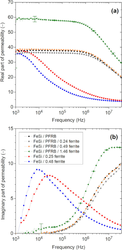
One really important thing to notice in the above plot is that even at relatively low frequencies of 10 kHz ferrite cores have a relatively low real component, for their permeability{: style="color: rgb(0,255,0)"}. Lower values of the real component indicate higher losses, therefore, ferrite cores tend to be relatively poor magnetic conductors; as such this is one among a few reasons magnetic circuits tend to be significantly more lossy than their electric circuit equivalent and are not used very often.
As a general rule the complex permeability{: style="color: rgb(0,255,0)"} can not be easily determined mathematically and it must be measured for a particular material at a specific frequency to find out what it is. However, much like electric loss tangent, once we know the complex permeability{: style="color: rgb(0,255,0)"} of a material at a particular frequency we can calculate its magnetic loss tangent with the following equation7.
$$ \tan{(\delta_e)} = \frac{\mu''}{\mu'} \label{maglosstan}$$
Where
\(\mu'\) and \(\mu^{\prime\prime}\) are components of the complex permeability{: style="color: rgb(0,255,0)"}, \(\color{permeability}\mu\color{normal}\) of the material such that.
$$ \color{permeability}\mu\color{normal} = \color{permeability}\mu' - j\mu''\color{normal} $$
However notice here that equation \(\eqref{maglosstan}\) does not include a conductivity term or an angular frequency term as it did with our dielectric loss tangent, equation \(\eqref{dieleclosstan}\). The complex permeability{: style="color: rgb(0,255,0)"} is still dependent on the frequency it is measured at, so we haven't actually eliminated our \(\omega\) term, it is just that now it happens to be rolled into the \(\color{permeability}\mu\color{normal}\) term indirectly. However the conductivity term is missing due to a more nuanced reason. If we were trying to determine the loss tangent of an electrical inductor with a ferrite core then the equation would, in fact, look much like our equation for dielectric loss tangent \(\eqref{diaelectloss}\); it would use the complex permeability{: style="color: rgb(0,255,0)"}, \(\color{permeability}\mu\color{normal}\), instead of complex permittivity{: style="color: rgb(255,0,0)"}, \(\color{permittivity}\varepsilon\color{normal}\), and would use resistivity, \(\rho\), instead of conductivity, \(\sigma\), but otherwise would look similar and include a term relating the DC resistance{: style="color: rgb(114,0,172)"} of the component. However in the case of an electrical inductor the resistivity term is intended to account for the DC resistance{: style="color: rgb(114,0,172)"} across the inductor, and thus the resistivity is due to the copper itself, and not the resistivity of the ferrite core. This makes it semantically a bit different than the case of a capacitor where the plates are electrically connected to the dielectric and thus the conductivity of the dielectric itself determines DC resistance{: style="color: rgb(114,0,172)"}. In the case of an inductor the DC resistance{: style="color: rgb(114,0,172)"} of the ferrite core does not effect the DC resistance{: style="color: rgb(114,0,172)"} of the inductor itself. However despite this fact the DC resistance{: style="color: rgb(114,0,172)"} of the ferrite core is not absent from our magnetic loss tangent equation \(\eqref{maglosstan}\), it still plays a role but in a very different way, it is reflected in the complex permeability{: style="color: rgb(0,255,0)"} itself, \(\color{permeability}\mu\color{normal}\), instead. As mentioned earlier one of the properties that effects the complex permeability{: style="color: rgb(0,255,0)"} is loss due to eddy currents{: style="color: rgb(0, 255, 221)"}; this is proportional to the conductivity of the material; materials with low conductivity/high resistivity having less loss due to eddy currents{: style="color: rgb(0, 255, 221)"}7. This is where conductivity/resistivity is hiding inside our complex permeability{: style="color: rgb(0,255,0)"}. However the effects are more complicated than the dielectric case because the magnitude of the eddies are also influenced by frequency. Also keep in mind we are talking about a magnetic circuit here, therefore, the changing magnetic field is considered directly when talking about magnetic resistance{: style="color: rgb(114,0,172)"} of a material, and the cause of the changing magnetic field may be manifold; it may be caused by an electrical inductor just as easily as it may be caused by a permanent magnet. Therefore the DC resistance{: style="color: rgb(114,0,172)"} of an electrical inductor, which is normally a consideration in determining an electrical inductors loss tangent, isn't relevant here. In short, we only care about the magnetic loss tangent as represented by equation \(\eqref{maglosstan}\) without some of the complexities we faced when dealing with the dielectric loss tangent.
As stated earlier this basically means that good magnetic conductors, meaning low loss, need to have both high electrical resistivity and a complex permeability{: style="color: rgb(0,255,0)"} with a high real component. Not many materials naturally have both these qualities so ferrite cores are produced by encapsulating iron granuels in a resistive coating and then pressing it into the desired shape for the core. This gives it a unique combination of permeability{: style="color: rgb(0,255,0)"} and resistance{: style="color: rgb(114,0,172)"}. The following chart shows the relationship between permeability{: style="color: rgb(0,255,0)"} and resistance{: style="color: rgb(114,0,172)"} of several materials to illustrate the uniqueness of ferrite core materials.
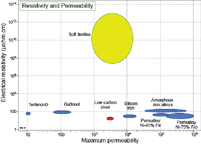
In the same way that our electrical loss tangent angle was represented as the angle relative to the negative reactive axis in the complex plane our magnetic loss tangent angle is represented by the angle in the complex plane relative to the positive reactive axis as can be seen in the following diagram.

Notice from the above diagram we are no longer calling the real portion of the complex vector ESR as we did with a capacitor. It is now referred to as magnetic resistance{: style="color: rgb(114,0,172)"} and represented by \(\color{resistance}R_m\color{normal}\). Similarly the earlier loss tangent equation, equation \(\eqref{losstan}\), remains the same except that \(\color{resistance}R_{_{ESR}}\color{normal}\) is replaced with \(\color{resistance}R_m\color{normal}\). Another thing to take note of here is that earlier in our table of duals we pointed out that magnetic resistance{: style="color: rgb(114,0,172)"} is measured in siemens, instead of ohms, which is the reciprocal of ohms. You may think that means we need to take the reciprocal of the ESR to get the magnetic resistance{: style="color: rgb(114,0,172)"}, however that is not the case. Remember that in both a dielectric as well as in a ferrite core or other material, that a higher resistivity of the material results in a lower ESR. In other words the ESR has an reciprocal relationship to the materials DC resistance{: style="color: rgb(114,0,172)"}. This is where the reciprocal relationship in the units comes from and is therefore already represented in the equations without needing to take the reciprocal when dealing with magnetic circuits.
Similarly in the above diagram the \(\color{reactance}X_m\color{normal}\) component would be our magnetic reactance{: style="color: rgb(45,177,93)"}. Much like magnetic resistance{: style="color: rgb(114,0,172)"} the magnetic reactance{: style="color: rgb(45,177,93)"} has a reciprocal relationship with its electrical dual; we see a similar relationship between electrical inductive reactance{: style="color: rgb(45,177,93)"} and electrical capacitive reactance{: style="color: rgb(45,177,93)"}. Remember earlier when we said that the magnetic loss tangent is taken relative to the positive reactive axis and the electric loss tangent is taken relative to the negative reactive axis. This presented itself in equations such as equation \(\eqref{losstan}\) as taking the absolute value of the reactance{: style="color: rgb(45,177,93)"}. Because reactance{: style="color: rgb(45,177,93)"} is the imaginary{: style="color: rgb(251,0,29)"} component of the complex impedance{: style="color: rgb(18, 110, 213)"}, the difference in sign between the negative reactance{: style="color: rgb(45,177,93)"} of a capacitor and the positive reactance{: style="color: rgb(45,177,93)"} of an inductor is due to a reciprocal relationship; remember the reciprocal of the imaginary{: style="color: rgb(251,0,29)"} number is its negative. Consider the equations for determining the impedance{: style="color: rgb(18, 110, 213)"} of an electric capacitor, or that of an inductor, they are effectively reciprocals of each other.
$$ \color{impedance}Z_{_C}\color{normal} = \color{impedance}\frac{1}{\omega C j}\color{normal} = \color{reactance}-\frac{1}{\omega C}\color{imaginary}j\color{normal}$$
$$ \color{impedance}Z_{_L}\color{normal} = \color{reactance}\omega L\color{imaginary} j\color{normal} $$
The same reciprocal relationship we see between electrical resistance{: style="color: rgb(114,0,172)"} and magnetic resistance{: style="color: rgb(114,0,172)"} is likewise baked into the relationship between electrical reactance{: style="color: rgb(45,177,93)"} and magnetic reactance{: style="color: rgb(45,177,93)"} by virtue of the fact that both are represented in their positive forms by way of taking the absolute values in our equations. Since magnetic impedance{: style="color: rgb(18, 110, 213)"} is the simple addition of our magnetic resistance{: style="color: rgb(114,0,172)"} and magnetic reactance{: style="color: rgb(45,177,93)"}, it too has a similar reciprocal relationship with electrical impedance{: style="color: rgb(18, 110, 213)"} as its components have. It is for this reason that magnetic resistance{: style="color: rgb(114,0,172)"}, * magnetic reactance*{: style="color: rgb(45,177,93)"}, and magnetic impedance{: style="color: rgb(18, 110, 213)"} all have the reciprocal unit of the ohm, the siemen.
Now that we got that out of the way we can take the final steps in showing how we can go from the complex permeability{: style="color: rgb(0,255,0)"} of a material at a certain frequency to actually determining its magnetic resistance{: style="color: rgb(114,0,172)"}. One way we can do this is use the equation for the ideal capacitance{: style="color: rgb(255, 127, 0)"} from equation \(\eqref{idealcap}\) and then use this to calculate \(\color{reactance}\mathcal{X}\color{normal}\). We can then use the same process we used earlier in electric capacitors to find the resistance{: style="color: rgb(114,0,172)"}.
$$ \color{reactance}\mathcal{X}\color{normal} = \frac{1}{\omega \color{capacitance}\mathcal{C}\color{normal}} \label{finalabs}$$
$$ \tan{(\delta_m)} = \frac{\color{resistance}\mathcal{R}\color{normal}}{|\color{reactance}\mathcal{X}\color{normal}|} $$
$$ \color{resistance}\mathcal{R}\color{normal} = |\color{reactance}\mathcal{X}\color{normal}| \cdot \tan{(\delta_m)} $$
$$ \color{resistance}\mathcal{R}\color{normal} = \left\lvert\color{reactance}\frac{1}{\omega \mathcal{C}}\color{normal}\right\rvert \cdot \tan{(\delta_m)} $$
$$ \color{resistance}\mathcal{R}\color{normal} = \left\lvert\color{reactance}\frac{1}{\omega C}\color{normal}\right\rvert \cdot \frac{\mu''}{\mu'} $$
$$ \color{resistance}\mathcal{R}\color{normal} = \frac{\mu''}{\omega \color{capacitance}\mathcal{C}\color{normal}\mu'} $$
Similarly we can now substitute in equation \(\eqref{idealcap}\) and get our equation relative to physical dimensions.
$$ \color{resistance}\mathcal{R}\color{normal} = \frac{\mu''}{\omega \color{capacitance}(\mu'' \frac{S}{L})\color{normal} \mu'} $$
$$ \color{resistance}\mathcal{R}\color{normal} = \color{resistance}\frac{\mu''L}{\omega\mu''\mu'S}\color{normal} $$
$$ \color{resistance}\mathcal{R}\color{normal} = \color{resistance}\frac{L}{\omega\mu'S}\color{normal} $$
We can also do the same substitution of equation \(\eqref{idealcap}\) on \(\mathcal{X}\) from equation \(\eqref{finalabs}\) as well if we want to determine the reactance{: style="color: rgb(45,177,93)"} component in order to construct the full impedance{: style="color: rgb(18, 110, 213)"}.
$$ \color{reactance}\mathcal{X}\color{normal} = \frac{1}{\omega \color{capacitance}(\mu'' \frac{S}{L})\color{normal}} $$
$$ \color{reactance}\mathcal{X}\color{normal} = \color{reactance}\frac{L}{\omega \mu'' S}\color{normal} $$
Therefore our full impedance{: style="color: rgb(18, 110, 213)"} would be
$$ \color{impedance}\mathcal{Z}\color{normal} = \color{resistance}\mathcal{R}\color{normal} + \color{reactance}\mathcal{X} \color{imaginary}j\color{normal} $$
$$ \color{impedance}\mathcal{Z}\color{normal} = \color{resistance}\frac{L}{\omega\mu'S}\color{normal} - \color{reactance}\frac{L}{\omega \mu'' S} \color{imaginary}j\color{normal} \label{finalimpcomplex} $$
That's all there is too it; we now have our complex impedance{: style="color: rgb(18, 110, 213)"}. We can also pull out our permeability{: style="color: rgb(0,255,0)"} values and change that back into a complex permeability{: style="color: rgb(0,255,0)"} for a more compact equation, but it is usually more helpful to keep it in the complex number form above. But just to show that relationship we would do that as follows
$$ \color{impedance}\mathcal{Z}\color{normal} = \frac{L}{\omega S} \cdot \color{permeability}( \mu' - \mu'' j)\color{normal} $$
$$ \color{impedance}\mathcal{Z}\color{normal} = \frac{L}{\omega S} \cdot \color{permeability}\mu\color{normal} \label{finalimp}$$
Where
\(\color{impedance}\mathcal{Z}\color{normal}\) is the complex magnetic impedance{: style="color: rgb(18, 110, 213)"} of the component,
\(L\) is the length of the component,
\(S\) is the cross sectional area of the component,
\(\omega\) is the angular frequency of the signal, and
\(\color{permeability}\mu\color{normal}\) is the absolute complex permeability{: style="color: rgb(0,255,0)"} of the material.
Keep in mind in the above equations the vertical bars that typically mean absolute value are surrounding a complex number, in that case it means to take the magnitude of the complex number. That effectively means dropping the imaginary{: style="color: rgb(251,0,29)"} number and taking the absolute value.
For the sake of clarity lets show how you can derive the same equation for magnetic impedance{: style="color: rgb(18, 110, 213)"} using the non-idealized form of the equation for capacitance{: style="color: rgb(255, 127, 0)"} shown in equation \(\eqref{realcap}\). Recall in this case the imaginary{: style="color: rgb(251,0,29)"} number will be part of our complex capacitance{: style="color: rgb(255, 127, 0)"} so while equation \(\eqref{finalabs}\) was for reactance{: style="color: rgb(45,177,93)"}, since it lacked the imaginary{: style="color: rgb(251,0,29)"} number, now the same equation represents impedance{: style="color: rgb(18, 110, 213)"} instead when used with a complex capacitance{: style="color: rgb(255, 127, 0)"} because our complex capacitance{: style="color: rgb(255, 127, 0)"} now provides the imaginary{: style="color: rgb(251,0,29)"} number.
$$ \color{impedance}\mathcal{Z}\color{normal} = \frac{1}{\omega \color{capacitance}\mathcal{C}\color{normal}} $$
$$ \color{impedance}\mathcal{Z}\color{normal} = \frac{1}{\omega \cdot \color{capacitance}(\mu \frac{S}{L})\color{normal}} $$
$$ \color{impedance}\mathcal{Z}\color{normal} = \frac{L}{\omega \color{permeability}\mu\color{normal} S} $$
$$ \color{impedance}\mathcal{Z}\color{normal} = \frac{L}{\omega S} \cdot \color{permeability}\mu\color{normal} $$
At this point our equation is identical to equation \(\eqref{finalimp}\) so it should be clear that this alternative approach works as well. It should also be clear that if we continued to expand the equation and put it in complex number form, as we did with equation \(\eqref{finalimpcomplex}\), we would see the imaginary{: style="color: rgb(251,0,29)"} number we expect come out of the \(\color{permeability}\mu\color{normal}\) argument. So this also serves to demonstrate nicely what I mentioned earlier how when using the real-world equation for a capacitor with complex capacitance{: style="color: rgb(255, 127, 0)"}; we do not need to add the imaginary{: style="color: rgb(251,0,29)"} number back in manually as this is already baked into the complex value of \(\color{permeability}\mu\color{normal}\) for us.
Examples of Magnetic Circuits
This section I just want to devote to showing some sketches of simple magnetic circuits that show how any electric circuit can have a magnetic circuit dual. Keep in mind these may not be particularly practical in real life, generally the electrical equivalent will be more efficient. The only purpose is to show that every electric circuit can be represented with a magnetic circuit dual.
DC Magnetic Lamp
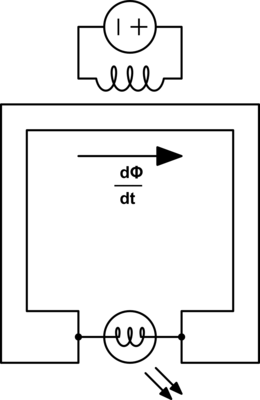
In this circuit we have an ideal voltage{: style="color: rgb(181, 181, 98)"} source connected to an inductor, which will produce a magnetic field that will constantly increase. This which will give us a magnetic current{: style="color: rgb(0, 255, 221)"} that flows consistently in one direction and remains constant. Keep in mind in real life the current{: style="color: rgb(0, 255, 221)"} through the inductor will also increase steadily, so while a real life version of this circuit will work for a short time, eventually you will see smoke and fire once the current{: style="color: rgb(0, 255, 221)"} gets too high for the inductor or voltage{: style="color: rgb(181, 181, 98)"} source to handle. The purpose in sharing this is to show that DC current{: style="color: rgb(0, 255, 221)"} does work in theory in a magnetic circuit, even if it isn't practical.
In this circuit, like other circuits, the wires are represented by the rectangular path. These would be made out of iron ferrite or plain iron. The lamp at the bottom of the circuit, however, would not be any ordinary light bulb. A light bulb in an electric circuit is just a resistive component that has its resistance{: style="color: rgb(114,0,172)"} selected to produce a specific power. Electric lamps work by heating due to their electrical resistance{: style="color: rgb(114,0,172)"} until the heat is enough to make the element glow white hot, and thus produce light. In a magnetic circuit this would be no different, a lamp would just be a block of material with a specifically chosen magnetic resistance{: style="color: rgb(114,0,172)"} such that it would convert the magnetic energy to heat at such a rate that it would glow white hot and produce light.
If you think about it an induction furnace is in some ways very similar to this circuit; it uses magnetic energy to heat up a piece of metal untill it turns white hot and glows with light. The only differences are that an induction furnace uses an AC magnetic current{: style="color: rgb(0, 255, 221)"} instead of DC and it it heats the material to the point of melting it. In a lamp you'd want to heat it enough to get it white hot but not so much that it would actually melt of course.
Magnetic High-pass Filter
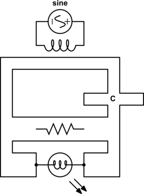
Here we have a simple magnetic bandpass filter where the magnetic lamp presents a resistance{: style="color: rgb(114,0,172)"} and would be factored into the component values. We added a magnetic capacitor in series with the lamp; there is also a horizontal connection just before the lamp representing a magnetic resistor acting as the resistive component to form the high-pass filter. If these were ideal components then a DC magnetic current{: style="color: rgb(0, 255, 221)"} would result in the lamp not lighting at all, and as the frequency of the sine wave generator increased the lamp would glow increasingly brighter.
Magnetic Oscillator and Bandpass Filter
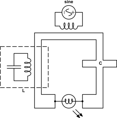
Finally this is the schematic for a magnetic oscillator or bandpass filter, depending on how it is used. If the power source is a sine wave generator then as the frequency approaches the resonance between the magnetic capacitor and the magnetic inductor the lamp would glow brighter; as it goes below or above the resonance the lamp would dim.
This would also work as an oscillator in the sense that if the sine wave generator produced a pulse instead of a steady sine wave, then the energy would oscillate between the capacitor and the inductor in the circuit at their resonant frequency until all the energy is dissipated by the lamp.
Permanent magnets as a Power Source
One final related point I wanted to make was on the topic of using permanent magnets as a DC power source in a magnetic circuit. Typically permanent magnets can not do work. This is because the energy stored in their magnetic field, in order to be consumed, must deplete the magnetic field. Just as an inductor would stop acting as an electromagnet if the energy in its magnetic field were consumed, so would a permanent magnet need to become demagnetized in order to consume the energy in its magnetic field. Since permanent magnets don't usually spontaneously become demagnetized during ordinary use it isn't typically the case that they can provide any power on their own when stationary, or indeed do any work at all.
However a permanent magnet's field does contain energy and under some special circumstances that energy can be extracted, though it wouldn't be practical to do so or to use them an energy source, it is as best a curiosity to demonstrate how this is possible. In the real world the energy extracted would not be significant enough to be practical. None the less, the energy that is stored, and thus able to be recovered, from a permanent magnet's magnetic field is exactly equal to energy delivered by an inductor that has a current{: style="color: rgb(0, 255, 221)"} going through it such that the field strength of the inductor is equal to that of the magnet. In both these cases the amount of power they could deliver to a circuit, given the correct circumstances, would be entirely equivalent.
In the case of the inductor, as we already illustrated, all that would be necessary would be to take the charged inductor, make sure it is wound around the iron wiring of our magnetic circuit, and then let the magnetic field collapse by cutting the current{: style="color: rgb(0, 255, 221)"} to the inductor. The collapsing magnetic field would cause the flux in the magnetic circuit to decrease at a constant rate and thus produce a DC magnetic current{: style="color: rgb(0, 255, 221)"} until the energy in the inductor is exhausted.
Similarly one could insert a permanent magnet of equivalent field strength into a gap cut out of the iron wiring of the magnetic circuit and let the field of the permanent magnet collapse creating an identical DC magnetic current{: style="color: rgb(0, 255, 221)"}. How do you get the field of a permanent magnet to collapse you may ask? Simple, just heat it up past a critical temperature, called the curie point, at that temperature the magnet looses its ferromagnetic properties and the field around it will collapse and provide all the same energy as the inductor did.
Now your first thought might be that the heat involved to get the magnet to the curie point is in fact the source of the energy and not the magnetic field itself. But that isn't the case and can be easily demonstrated by the fact that the energy extracted from such a scenario would be identical regardless of the amount of energy needed to raise the temperature of the magnet to the curie point. A simple thought experiment can demonstrate this. Imagine you had a magnet where the curie point of the magnet is infinitesimally higher than the ambient temperature in the room you are in and setup the circuit as previously described. At this point you could simply touch the magnet and the added warmth from your body will raise its temperature ever so slightly past the curie point. This would represent an infinitesimal amount of energy transferred into the magnet, and thus the energy to do so would be negligible. None the less at this point the magnetic field of the magnet would begin to collapse and the energy of the magnet would be successfully extracted as DC magnetic current{: style="color: rgb(0, 255, 221)"}.
You could literally run circuits off the energy stored in permanent magnets... well as much as you could from a charged inductor, which is to say, you wont be able to deliver all that much power to really be useful as a power source. But hey, still cool to know that magnets can be used as a power source all the same. Just don't go getting any crackpot ideas about over unity devices or infinite energy. There is a finite and small amount of energy in a magnet and once you use it up, its gone, so no infinite energy anytime soon I'm afraid.
Special Thanks
Special thanks to the following people for helping me proof-read and edit this article prior to its release:
- Faith Aydin - He submited several corrections through gitlab catching numerous spelling and gramatical errors.
Citations
-
González, G. G., & Ehsani, M. (2018). "Power-Invariant Magnetic System Modeling", International Journal of Magnetics and Electromagnetism, 4(1), 1-9. doi:10.35840/2631-5068/6512. ISSN 2631-5068. ↩︎ ↩︎ ↩︎ ↩︎ ↩︎
-
Popov, V. P. (1985). The Principles of Theory of Circuits (in Russian). M.: Higher School. ↩︎ ↩︎ ↩︎
-
Mohammad, Muneer (2014-04-22). An Investigation of Multi-Domain Energy Dynamics (PhD thesis). ↩︎ ↩︎
-
Lambert, M., Mahseredjian, J., Martinez-Duro, M., & Sirois, F. (2015). Magnetic Circuits Within Electric Circuits: Critical Review of Existing Methods and New Mutator Implementations. IEEE Transactions on Power Delivery, 30(6), 2427–2434. doi:10.1109/tpwrd.2015.2391231](https://doi.org/10.1109/tpwrd.2015.2391231) ↩︎
-
[https://www.ece.rutgers.edu/~orfanidi/ewa/ch01.pdf](Maxwell's Equations, Rutgers) ↩︎ ↩︎
-
"Considerations for a High Performance Capacitor". Archived from the original on 2008-11-19. ↩︎
-
Hong, Y.-K., & Lee, J. (2013). Ferrites for RF Passive Devices. In Recent Advances in Magnetic Insulators – From Spintronics to Microwave Applications (pp. 237–329). Elsevier. doi:10.1016/b978-0-12-408130-7.00008-3 ↩︎ ↩︎ ↩︎