Restricted Logarithmic Growth with Injection
 Jeffrey P. Freeman
May 30, 2016
11 min read
Jeffrey P. Freeman
May 30, 2016
11 min read
TL;DR An exploration of the Verhulst logistic growth model, from unrestricted exponential growth to restricted logarithmic growth, culminating in a novel extension that adds an artificial injection term to account for advertising, conservation breeding, and other external accelerants. The Logistic Function, sometimes with modifications, has been used successfully to model a large range of natural systems. Some examples include bacterial growth, tumor growth, animal populations, neural network transfer functions, chemical reaction rates, language adoption, and diffusion of innovation, to name a few.
An exploration of the Verhulst logistic growth model, from unrestricted exponential growth to restricted logarithmic growth, culminating in a novel extension that adds an artificial injection term to account for advertising, conservation breeding, and other external accelerants.
The Logistic Function, sometimes with modifications, has been used successfully to model a large range of natural systems. Some examples include bacterial growth, tumor growth, animal populations, neural network transfer functions, chemical reaction rates, language adoption, and diffusion of innovation, to name a few. The real world applications are simply staggering.
Because of the utility of this powerful little equation it has lead me to investigate more thoroughly how it works, and how it can be applied to novel innovations.
There have been many contributions that have led to numerous variations of the Logistic function. One that struck my attention in particular is the Verhulst Equation, sometimes referred to descriptively as the "Restricted Logarithmic Growth Function", or simply "Logistic Growth Function". It is used in ecology to model the expected growth of a population while taking into consideration that resources, such as food, are finite, resulting in a maximum sustainable population, called the carrying capacity. The model demonstrates an exponential growth of the population when it is significantly below this carrying capacity, but as the population approaches the carrying capacity, and resource competition increases, the growth rate slows asymptotically. The Verhulst Equation has been tested against numerous real world populations, including Seals and Elk, and has been shown to be a relatively accurate model.
Of course the Verhulst Equation isn't limited to modeling animal populations, it has also been successfully used to model diffusion of innovation. In this sense it can be used to represent how ideas spread throughout a population. It is this particular application that was most interesting to me.
Unrestricted Exponential Growth
As with any complex idea we have to start with the basics. Whether we are talking about an idea or an organism, if it is capable of spreading through multiplying itself, then obviously the more it spreads, the faster it will spread. You start out with one, which turns into two, then four, then eight, in just a few iterations you will have billions; if there is nothing to impede the growth, then it will follow an exponential curve.
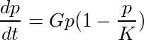
We can model this sort of growth quite simply; the rate at which new members of the population will be observed can be represented as the growth rate, G, multiplied by the population, p.
You will notice in the above equation that there is a derivative on the left hand side of the equation. The equation can therefore be read as "The rate of change in the population for each unit of time is equal to the growth rate multiplied by the current population". If the population is seen to double each year, for example, then time would have a unit of years, and G would be 2.
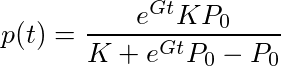
Of course the equation becomes much more useful if we can get rid of the derivative and simply express the total population at any point in time. To do that we integrate the equation, while solving for p and we arrive at the following equation.
Here the variable e is Euler's constant, and P0 is our constant of integration which represents the population when time, t, is equal to 0.
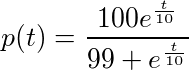
To help visualize whats going on lets try some arbitrary values for our constants. Lets suppose the growth rate is 0.1, and our P0 is 1. This would represent a initial population with only one member capable of replicating once for every 10 units of time that have passed. If we plug these values in and simplify we arrive at the following equation.
It is immediately obvious this is an exponential function, nothing too special about that. We can see from the graph below that the population would continue to grow exponentially and unrestricted.

Restricted Logarithmic Growth
Of course in the real world it is rare that anything will truly grow in an unrestricted manner. Space is finite, resources are finite, eventually everything must stop growing. This brings us to the Restricted Logarithmic Growth model, also called the Verhurst Equation.
Verhurst recognized that, at least amongst animals, resources are limited. When unlimited resources are available to an organism it will grow and reproduce unrestricted. However as the population grows resources become scarce. The more scarce the resources, the greater the restriction on growth and reproduction, and this effect will scale according to the proportion of the resources which are free. Therefore as the population reaches the carrying capacity of the environment then the growth rate should approach 0 in a linear fashion.
Therefore if we take the growth rate equation from before, we can add an additional term to represent the availability of resources.
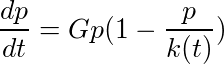
In the above equation we can see that we multiply by a term that scales proportionally to the population. The term will evaluate to 1 when the population is 0, and will approach 0 as the population approaches the carrying capacity, represented as k(t). This is where the population's growth restriction is represented.
Before we can actually solve the equation above, we have to actually know what the k(t) function evaluates to; after all we can't perform integration on a function if we don't know what that function is. So lets just assume the carrying capacity is a constant we will call K.
At this point we can solve for p and integrate the equation as before. This will give us an equation which models the total population as a function of time.
The above equation is usually what people refer to when they talk about the Verhulst equation, but it might help to see what it looks like with some actual values plugged in for the constants. Lets pick similar values with a growth rate, G, of 0.1, an initial population, P0 of 1, and a carrying capacity, K, of 100.
Once we plug these values in and simplify we arrive at the above equation. It is a specific form of the Logistic Function. If we graph that we will get the following graph.

In the above graph the dotted horizontal orange line represents the carrying capacity, K. This is of course a constant with a value of 100. We can see that early on the population has what appears to be an exponential growth pattern, but as it begins to approach the orange dashed line it asymptotically tappers off. Of course as time approaches infinity (the x axis) then the population approaches the carrying capacity.
Time-varying Carrying Capacity
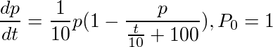
If we want to play with this equation a bit more we can make things more complex (and fun) by picking a carrying capacity that actually changes with time. If we go back to the original growth rate equation we can make k(t) a function equal to (t/10)+100, rather than a constant. If we do this, and keep the growth rate and P0 constants the same as before, then we will get the following equation.
Again we can solve for p, integrate, and simplify and we will arrive at the following equation.
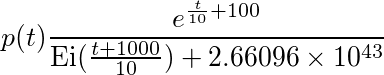
In the above equation Ei is the Exponential Integral Function. If you don't know what that is don't worry, we can just graph the equation below to get a better understanding of how it behaves.

You can see the equation behaves similarly in this graph as in the last graph. The only exception is that the carrying capacity starts at 100 and slowly increases over time. As this happens the population also increases to match the carrying capacity without ever exceeding the carrying capacity. Pretty much how we would expect it to work.
Restricted Logarithmic Growth with Injection
This is where the lessons of history end, and my own contribution begins. I was left considering the effects of a modern world and how they could be reflected in the Verhurst model.
As I mentioned in the introduction the Verhurst equation has since been used in countless applications outside of ecology models. One that was particularly interesting is that it has been used successfully to model the Diffusion of Innovation. Essentially it can accurately describe the adoption of an idea within a population. For example it can model the proliferation of linguistic changes such as the change in the spelling of a word, or even the adoption of an entirely new word.
All of this, of course, has implications in marketing where the marketing penetration of a product can spread through word of mouth alone and can therefore be modeled using the Verhurst equation. But how could we use this to also account for the effects of advertising, which can often act as an accelerant to the spreading of an idea that is still primarily driven by word of mouth. Thats when inspiration struck.
If we accept that ideas spreading through word of mouth will often fit a model similar to population growth, then advertising is a bit like artificially injecting new members into a population as it grows. The advertising acts as a jump start to the population growth, accelerating it, and magnifying the effects that would be seen from word of mouth alone.
If I could incorporate this effect into the model not only could it be used for modeling product adoption, but conservationism efforts as well. It is not uncommon for conservationists to breed in captivity and then release in the hopes of supplementing a specie's population. In this sense it would be modeled with the same artificial injection.
In fact almost all the examples given earlier where the Verhurst model has been used in the past could potentially benefit from this addition. Consider chemical reactions; an artificial injection factor could represent the effects of slowly adding new reactants to a reaction as it progresses.
So I had to figure out where this new function might fit in. When we go back and take a look at our original differential growth rate equation we have two terms, the left hand term represented the unrestricted growth rate, and the right hand term represented the constraint on growth as the resource contention grows. So all it really takes is adding an injection factor to the left hand term. The new equation looks like the following.
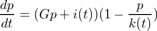
You will notice in the above equation all we did was add the new injection function, shown as i(t). This is just the number of artificially injected members of the population per unit of time. By representing it as a function it can of course change over time such that we can inject a varying number of members over time.
It is important to keep in mind that this injection is still scaled by the right hand term. The more resource contention there is the less effective the injection is likely to be. If we consider the earlier example of breeding animals in captivity and releasing them into the wild then this represents the fact that if resources are scarce many of the animals released are likely to die of starvation before they have a chance to have children. In the case of advertisement, or Diffusion of Innovation in general, then it is reasonable to expect that the more people that know about an idea the harder it would be for your advertisements to reach new people who have yet to hear word of it. If Pepsi plays a commercial on TV, for example, you might expect the vast majority of people who see it to already know about the Pepsi brand.
As before if we want to play around with the equation a bit to see how the model plays out we are going to have to create some definitions for our functions.
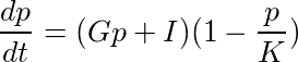
For the sake of simplicity we turned our injection function, i(t), into the constant I, and the carrying capacity, k(t), into the constant K. This just gives us something to play with and allows us to solve for p and integrate in the following equation.
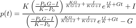
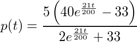
Now lets plug in some arbitrary values for our constants and see how it graphs out. Lets pick a value of 1/2 for I, 1/10 for G, 100 for K, and 1 for P0. If we plug these values in and simplify we arrive at the following equation.
Finally, lets graph the carrying capacity and growth model as before. In the graph below carrying capacity is once again represented by the dashed yellow line, and the solid blue line is the population. We can immediately notice that while the graph still has a logistic curve to it that the population grows significantly quicker in the beginning than with the other models, but despite the injection it still does not exceed the carrying capacity at any point.

While this model has yet to be tested against real world data I am hopeful that it will provide an accurate representation of an artificial population injection in growth models. I am looking forward to see how I and others might apply this and similar models to data in the future.
check_circleKey takeaways
-
- The Verhulst equation models restricted growth by introducing a carrying capacity that limits exponential expansion
- Time-varying carrying capacity allows modeling environments where resources change over time
- Adding an injection term to the growth rate equation accounts for external accelerants like advertising or conservation breeding
- Even with injection, the population remains bounded by the carrying capacity
- The extended model is applicable to marketing, ecology, chemical reactions, and diffusion of innovation
Data scientist, open-source innovator, and three-time founder who writes about graphs, radios, and the occasional impossibility. Allegedly just another data scientist. Say hello →